1. What is Gradient Descent?
Gradient Descent is an optimization algorithm which is used when training data models. Changing its parameters iteratively to minimize a given function to its local minimum.
2. Why do we need to use Gradient Descent?
The main reason why we need to use gradient descent is the computational complexity. From this Linear Regression post, we have the formula to find the solution of a loss function:
$$
\mathbf{w} = (\mathbf{X}\mathbf{X^T})^{-1} \mathbf{X}\mathbf{y}
$$
For example, matrix \(\mathbf{X}\) has \(m\) columns & \(n\) rows. In a machine learning algorithm you can end up with \(m > 10^3\) & \(n > 10^6\). The calculation to invert that matrix is expensive.
3. Gradient Descent algorithm

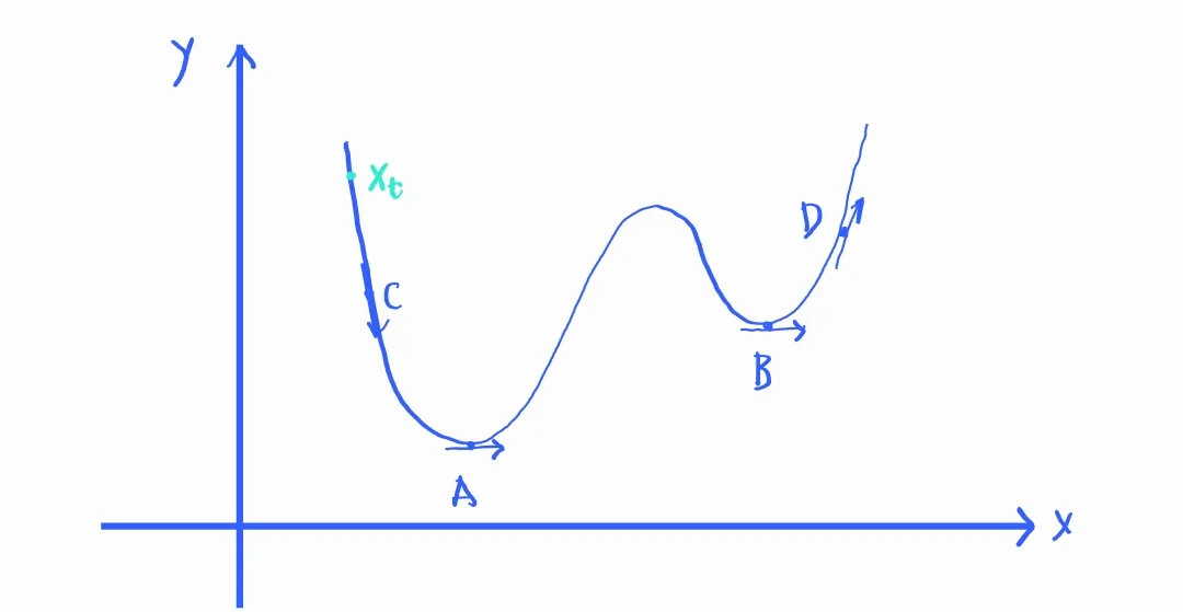
That function has two local minimum points (A, B) that have the derivative equal 0. A is called as global minimum point. The C point has the derivative < 0 & the D point has the derivative > 0.
Starting from a \(x_t\) point, after some loops, we need to find an algorithm to move \(x_t\) as close to A as possible. As you can see
- If the derivative of \(x_t\) > 0, we need to move \(x_t\) to the right.
- If the derivative of \(x_t\) < 0, we need to move \(x_t\) to the left.
From the above conditions, we have the function to move \(x_t\)
$$
x_{t+1} = x_t – \eta f'(x_t) ~~~~~~~~ (3.1)
$$
\(\eta\) is the learning rate.
4. A basic Python sample
A given function:
$$
\begin{align}
f(x) &= x^2 + sin(x) ~~~~~~~~ (4.1) \\
\Rightarrow f'(x) &= 2x + cos(x)
\end{align}
$$
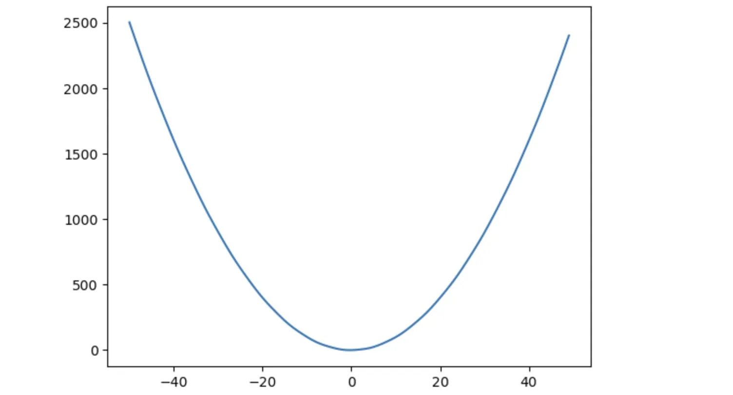
We will show that function on the chart by creating 100 points from -50 to 50
    import numpy as np
import matplotlib.pyplot as plt

def calc(x):
    return x**2 + np.sin(x)

# Create array of x points
xArr = list(range(-50, 50))
yArr = []

# Create array of y points
for item in xArr:
    y = calc(item)
    yArr.append(y)

plt.plot(xArr,yArr)
plt.show()

The logic to calculate derivative of (4.1) function:
    def derivative(x):
    return 2*x + np.cos(x)
Based on (3.1), we have the logic to calculate the gradient when having the learning rate & starting point. The logic will stop when the derivative approaches a value of approximately 0 (0.001). The function returns two values: an array of all points, the number of rounds.
    def gradient(rate, startX):
    arrayX = [startX]
    for round in range(100):
        nextX = arrayX[-1] - rate * derivative(arrayX[-1])
        if abs(derivative(nextX)) < 0.001:
            break
        arrayX.append(nextX)
    return (arrayX, round)
The full code to calculate the gradient when the learning rate = 0.1 & starting point = 5
    import numpy as np
import matplotlib.pyplot as plt

def calc(x):
    return x**2 + np.sin(x)

def derivative(x):
    return 2*x + np.cos(x)

def gradient(rate, startX):
    arrayX = [startX]
    for round in range(100):
        nextX = arrayX[-1] - rate * derivative(arrayX[-1])
        if abs(derivative(nextX)) < 0.001:
            break
        arrayX.append(nextX)
    return (arrayX, round)

(arrayX, round) = gradient(0.1, 5)

print('Points array:', arrayX)
print('Rounds:', round)
print('Solution: %f'%(arrayX[-1]))
print('Derivative: %f'%(derivative(arrayX[-1])))
The result is:
- Points array: [5, 3.9716337814536775, 3.2447915661588933, 2.6953012245767334, 2.2464463803687083, 1.859697572895399, 1.5162479761675645, 1.2075462506330112, 0.9305055901721205, 0.6846616106645871, 0.4702659792767276, 0.28706800359206847, 0.13374658623463562, 0.007890343974392533, -0.09368461196023423, -0.17450917011644537, -0.23808852386927765, -0.2876498753918038, -0.32601122551592154, -0.3555417152882604, -0.3781791778541007, -0.39547718987973746, -0.4086630351746791, -0.4186957211040709, -0.4263185765700088, -0.4321042877163536, -0.4364920823482641, -0.43981769128108905, -0.44233708309110803, -0.44424504020769906, -0.44568957081908495, -0.44678301861799863, -0.4476105865562553, -0.4482368535849964, -0.44871074389544563, -0.44906930869779466, -0.4493406000538505, -0.4495458523251541, -0.4497011366674418]
- Rounds: 38
- Solution: -0.449701
- Derivative: 0.001175
At the learning rate = 0.1, we can find the local minimum of (4.1) after 38 rounds. The next step, we will change the learning rate to 0.5 & see the result
- Points array: [5, -0.14183109273161332, -0.4949794099625081, -0.43998924528459094, -0.452378122012684, -0.4497050779971135]
- Rounds: 5
- Solution: -0.449705
- Derivative: 0.001165
After changing the learning rate, we can find the local minimum after 5 rounds. So choosing the learning rate will affect the calculation speed.
