Kien Duong

September 6, 2024

Neural Network

Neural Network is a machine learning program, or model, that makes decisions in a manner similar to the human brain, by using processes that mimic the way biological neurons work together to identify phenomena, weigh options and arrive at conclusions.

1. Introduction

1.1. Neuron (Node)

The basic unit of a neural network, analogous to a brain’s neuron. It receives inputs, processes them, and produces an output.

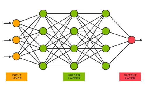
1.2. Input Layer

This is the first layer of the neural network, which receives the input data. Each node (or neuron) in the input layer corresponds to a feature in the dataset.

1.3. Hidden Layers

These layers sit between the input and output layers and perform most of the computations in the network. A neural network can have one or multiple hidden layers, and each layer consists of neurons connected to the previous and next layers.

1.4. Output Layer

This layer provides the final output of the neural network. The number of neurons in the output layer depends on the task.

For classification problems, it typically has as many neurons as there are classes.
For regression problems, it often has one neuron, providing a continuous value.

1.5. Weights and Biases

Weights represent the importance of each input in contributing to the output. They are adjusted during the training process to minimize the prediction error.
Biases are additional parameters in neurons that allow the model to fit the data better by shifting the activation function.

1.6. Activation Functions

These functions define how the weighted sum of inputs (plus bias) is transformed before passing it to the next layer.

1.7. Loss Function

This function measures the difference between the predicted output and the actual output (target). The goal of training is to minimize the loss function. Examples of loss functions are:

Mean Squared Error (MSE) for regression.
Cross-Entropy Loss for classification tasks.

1.8. Optimizer

The optimizer adjusts the weights and biases in order to minimize the loss function. E.g. Stochastic Gradient Descent (SGD)

1.9. Forward Propagation

In forward propagation, the input data is passed through the network layer by layer to compute the output. The input is transformed using weights, biases, and activation functions at each layer.

1.10. Backpropagation

Backpropagation is a key process in training the neural network. It involves computing the gradient of the loss function with respect to each weight in the network, allowing the optimizer to update the weights and minimize the loss. This is done using the chain rule of calculus.

1.11. Epochs, Batches, and Iterations

Epoch: One complete pass of the entire training dataset through the network.
Batch: A subset of the dataset used to update the weights during each training iteration.
Iteration: One update of the model’s parameters based on a batch of data.

2. Basic sample

The problem: Predicting Match Outcomes (Win, Loss, Draw)

2.1. Features (Inputs)

Let’s assume we have the following features for each football match:

Team 1: A rating or score representing the strength of team 1 (e.g., average player rating, win/loss ratio).
Team 2: A rating or score representing the strength of team 2.
Home Advantage: A binary value (1 if team 1 is playing at home, 0 otherwise).
Injuries: Number of injured players in team 1 and team 2.
Past Head-to-Head Results: Performance history between the two teams (e.g., win/loss/draw ratio).

2.2. Output (Predicted Result)

The network will predict whether team 1 will:

Win (Output = 1)
Lose (Output = -1)
Draw (Output = 0)

2.3. Structure of the Neural Network

Input Layer: 5 input features (Team 1 strength, Team 2 strength, Home advantage, Injuries, Head-to-head).
Hidden Layer: 4 neurons (can be increased for more complexity).
Output Layer: 3 neurons (representing probabilities of win, loss, or draw).

2.4. Forward Propagation

2.4.1. Input Layer

Input features: Team strengths, home advantage, injuries, head-to-head history.

2.4.2. Hidden Layer

Weights and biases connect the input to the hidden layer neurons.
Apply the ReLU activation function to each neuron to allow the network to learn non-linear patterns.

2.4.3. Output Layer

The output layer consists of 3 neurons. Use a softmax activation function to output probabilities for each class (win, loss, or draw).

2.5. Loss Function and Optimizer

Loss Function: Use categorical cross-entropy to measure the difference between the predicted and actual results (since we are predicting multiple categories: win, loss, draw).
Optimizer: Use Adam or SGD (Stochastic Gradient Descent) to minimize the loss function and adjust weights.

3. Python Code

3.1. Prepare the Dataset (features and labels)

The features:

Team 1 strength
Team 2 strength
Home advantage
Injuries team 1
Injuries team 2
Head-to-head

The dataset for 5 matches

    X = np.array([
    [85, 80, 1, 2, 1, 0.7],
    [78, 90, 0, 1, 3, 0.4],
    [82, 85, 1, 0, 0, 0.6],
    [90, 78, 1, 1, 2, 0.5],
    [88, 92, 0, 3, 2, 0.3],
], dtype=np.float32)

The labels:

Team 1 wins = [1, 0, 0]
Draw = [0, 0, 1]
Team 1 loses = [0, 1, 0]

    y = np.array([
    [1, 0, 0],
    [0, 0, 1],
    [0, 1, 0],
    [1, 0, 0],
    [0, 1, 0],
], dtype=np.float32)

3.2. Neural Network Model

We define a simple feedforward neural network using nn.Module

An input layer with 6 input neurons (since there are 6 features).
A hidden layer with 4 neurons (can be increased for more complexity).
An output layer with 3 neurons corresponding to the 3 possible outcomes (win, draw, or lose).
ReLU Activation: This is applied to the output of the hidden layer to introduce non-linearity.
Softmax Activation: The output layer uses softmax to output probabilities for each class (win, lose, or draw).

    class FootballNN(nn.Module):
    def __init__(self):
        super(FootballNN, self).__init__()
        self.fc1 = nn.Linear(6, 4)
        self.fc2 = nn.Linear(4, 3)

    def forward(self, x):
        x = torch.relu(self.fc1(x))
        x = torch.softmax(self.fc2(x), dim=1)
        return x

3.3. Optimizer (SGD)

Adjusts the weights based on a small portion of the data (or even individual samples) during each iteration.
The learning rate is set to 0.01, a hyperparameter that controls how much to adjust the model’s weights at each step.

    model = FootballNN()
loss_function = nn.CrossEntropyLoss()
optimizer = optim.SGD(model.parameters(), lr=0.01)

3.4. Training

We train the model over 1000 epochs:

Forward Pass: We pass the input features through the network to get predictions.
Loss Calculation: We calculate the loss between the predicted values and the actual labels using CrossEntropyLoss, which is appropriate for multi-class classification problems.
Backward Pass: The gradients are computed using backpropagation.
Weight Update: The optimizer (SGD) updates the weights using the computed gradients.

    epochs = 1000
for epoch in range(epochs):
    # Zero the gradients from the previous step
    optimizer.zero_grad()
    
    # Forward pass: Compute predicted y by passing X to the model
    output = model(X)
    
    # Compute the loss
    # CrossEntropyLoss expects class labels (0, 1, 2), so we convert y to labels
    loss = loss_function(output, torch.argmax(y, dim=1))
    
    # Backward pass: Compute gradients
    loss.backward()
    
    # Update weights using SGD
    optimizer.step()

    # Print the loss every 100 epochs
    if (epoch+1) % 100 == 0:
        print(f'Epoch {epoch+1}/{epochs}, Loss: {loss.item():.4f}')

3.5. Testing

Once the model is trained, we can use it to predict the outcome of a new match. In this case, we input the features of a new match and obtain the predicted probabilities for a win, draw, or loss.

    test_match = torch.tensor([[88, 85, 1, 2, 0, 0.6]], dtype=torch.float32)
prediction = model(test_match)
prediction_percent = prediction.detach().numpy() * 100

# Print the probabilities as percentages for Win, Draw, and Lose
print(f'Prediction (Win, Draw, Lose percentages): {prediction_percent[0][0]:.2f}% Win, {prediction_percent[0][2]:.2f}% Draw, {prediction_percent[0][1]:.2f}% Lose')ach().numpy()}')

The full source code:

    import torch
import torch.nn as nn
import torch.optim as optim
import numpy as np

# Step 1: Prepare the Dataset (features and labels)
# Features: [team 1 strength, team 2 strength, home advantage, injuries team 1, injuries team 2, head-to-head]
X = np.array([
    [85, 80, 1, 2, 1, 0.7],  # Match 1
    [78, 90, 0, 1, 3, 0.4],  # Match 2
    [82, 85, 1, 0, 0, 0.6],  # Match 3
    [90, 78, 1, 1, 2, 0.5],  # Match 4
    [88, 92, 0, 3, 2, 0.3],  # Match 5
], dtype=np.float32)

# Labels (win = [1, 0, 0], draw = [0, 0, 1], lose = [0, 1, 0])
y = np.array([
    [1, 0, 0],  # Team 1 wins
    [0, 0, 1],  # Draw
    [0, 1, 0],  # Team 1 loses
    [1, 0, 0],  # Team 1 wins
    [0, 1, 0],  # Team 1 loses
], dtype=np.float32)

# Convert the data to PyTorch tensors
X = torch.tensor(X)
y = torch.tensor(y)

# Step 2: Define the Neural Network Model
class FootballNN(nn.Module):
    def __init__(self):
        super(FootballNN, self).__init__()
        # Input layer (6 features) -> Hidden layer (4 neurons)
        self.fc1 = nn.Linear(6, 4)
        # Hidden layer -> Output layer (3 neurons for win, draw, lose)
        self.fc2 = nn.Linear(4, 3)

    def forward(self, x):
        # Pass input through the first fully connected layer and apply ReLU activation
        x = torch.relu(self.fc1(x))
        # Pass the result through the second fully connected layer and apply softmax activation
        x = torch.softmax(self.fc2(x), dim=1)
        return x

# Step 3: Initialize the model, define loss function, and use SGD optimizer
model = FootballNN()
# Using Cross-Entropy Loss as we have multiple classes (win, draw, lose)
loss_function = nn.CrossEntropyLoss()
# Using SGD (Stochastic Gradient Descent) optimizer with a learning rate of 0.01
optimizer = optim.SGD(model.parameters(), lr=0.01)

# Step 4: Training the Model
epochs = 1000
for epoch in range(epochs):
    # Zero the gradients from the previous step
    optimizer.zero_grad()
    
    # Forward pass: Compute predicted y by passing X to the model
    output = model(X)
    
    # Compute the loss
    # CrossEntropyLoss expects class labels (0, 1, 2), so we convert y to labels
    loss = loss_function(output, torch.argmax(y, dim=1))
    
    # Backward pass: Compute gradients
    loss.backward()
    
    # Update weights using SGD
    optimizer.step()

    # Print the loss every 100 epochs
    if (epoch+1) % 100 == 0:
        print(f'Epoch {epoch+1}/{epochs}, Loss: {loss.item():.4f}')

# Step 5: Testing the Model with New Data
test_match = torch.tensor([[88, 85, 1, 2, 0, 0.6]], dtype=torch.float32)
prediction = model(test_match)

# Convert the prediction values to percentages
prediction_percent = prediction.detach().numpy() * 100

# Print the probabilities as percentages for Win, Draw, and Lose
print(f'Prediction (Win, Draw, Lose percentages): {prediction_percent[0][0]:.2f}% Win, {prediction_percent[0][2]:.2f}% Draw, {prediction_percent[0][1]:.2f}% Lose')

The result:

    Epoch 100/1000, Loss: 1.0482
Epoch 200/1000, Loss: 0.8667
Epoch 300/1000, Loss: 0.8280
Epoch 400/1000, Loss: 0.9334
Epoch 500/1000, Loss: 0.7619
Epoch 600/1000, Loss: 0.7590
Epoch 700/1000, Loss: 0.7573
Epoch 800/1000, Loss: 0.7562
Epoch 900/1000, Loss: 0.7554
Epoch 1000/1000, Loss: 0.7548
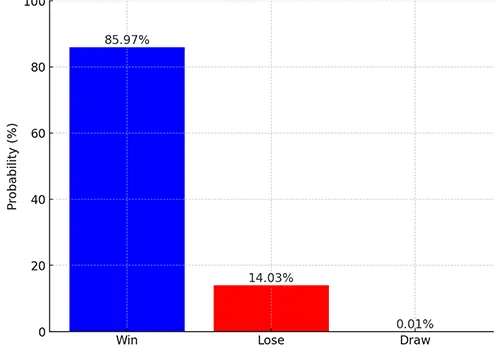
Prediction (Win, Draw, Lose percentages): 85.97% Win, 0.01% Draw, 14.03% Lose

This output shows that the model predicts a 85.97% chance of Team 1 winning, a 14.03% chance of Team 1 losing, and a 0.01% chance of a draw.