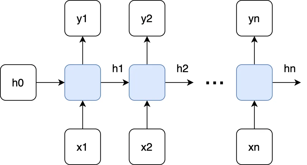
Backpropagation Through Time (BPTT) is a technique used to train recurrent neural networks (RNNs).

Recurrent Neural Network (RNN)

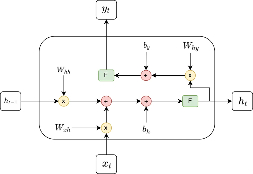
RNN time step
1. Forward Pass
\[ h_t = f(W_{xh} x_t + W_{hh} h_{t-1} + b_h) ~~~~~~~~~~ (1.1) \]
- is the weight matrix for the hidden state.
- is the weight matrix for the input.
- is the bias term.
- is the activation function (e.g. tanh or ReLU).
The output \(y_t\) at time step \(t\) is computed as:
\[ y_t = g(W_{hy} h_t + b_y) ~~~~~~~~~~ (1.2) \]
- \(W_{hy}\) is the weight matrix for the hidden-to-output layer.
- \(b_y\) is the output bias.
- \(g\) is the output activation function (e.g. softmax for classification).
2. Loss Function
\[ \mathcal{L}_{\text{total}} = \sum_{t=1}^{T} \mathcal{L}(y_t, \hat{y}_t) ~~~~~~~~~~ (2.1) \]
- \(y_t\) is the predicted output.
- is the target output.
3. Backpropagation Through Time (BPTT)
3.1. Calculate the gradients with respect to \(h_t\)
\[ \frac{\partial L}{\partial h_t} = \frac{\partial L_t}{\partial h_t} + \sum_{k=t+1}^{T} \frac{\partial L_k}{\partial h_k} \cdot \frac{\partial h_k}{\partial h_t} ~~~~~~~~~~ (3.1) \]
The above formula can be broken down into 2 parts:
3.1.1. Direct contribution of \(h_t\)
At time \(t\), the hidden state \(h_t\) influences the output \(y_t\) which is compared with the target output \(\hat{y}_t\) to compute the loss \(L_t\) at that specific time step.
\[ L_t = \text{Loss}(y_t, \hat{y}_t) \]
\[ \frac{\partial L_t}{\partial h_t} \]
Apply the chain rule:
\[ \frac{\partial L_t}{\partial h_t} = \frac{\partial L_t}{\partial y_t} \cdot \frac{\partial y_t}{\partial h_t} \]
- \( \frac{\partial L_t}{\partial y_t} \)
Based on Mean Squared Error (MSE)
\[ L_t = \frac{1}{2} (y_t – \hat{y}_t)^2 \]
\[ \Rightarrow \frac{\partial L_t}{\partial y_t} = y_t – \hat{y}_t \]
- \( \frac{\partial y_t}{\partial h_t} \)
Based on (1.2)
\[ \Rightarrow \frac{\partial y_t}{\partial h_t} = \frac{\partial y_t}{\partial (W_{hy} h_t + b_y)} \cdot \frac{\partial (W_{hy} h_t + b_y)}{\partial h_t} \]
\[ \Rightarrow \frac{\partial y_t}{\partial h_t} = g'(W_{hy} h_t + b_y) \cdot W_{hy} \]
- Combining:
\[ \Rightarrow \frac{\partial L_t}{\partial h_t} = (y_t – \hat{y}_t ) \cdot g'(W_{hy} h_t + b_y) \cdot W_{hy} ~~~~~~~~~~ (3.2) \]
3.1.2. Indirect contribution of \(h_t\)
In an RNN, each hidden state carries information about previous inputs. This information is passed along the sequence, allowing the RNN to capture patterns that depend on multiple previous inputs. However, this also means that each hidden state indirectly influences future hidden states, which affects future outputs and losses. When calculating gradients during training, we need to account for these indirect effects. E.g.
- Suppose we change the hidden state \(h_t\).
- This change will affect \(h_{t+1}\) (based on (1.1)), which then affects \(h_{t+2}\), and so forth, all the way to \(h_T\).
- As a result, each loss term \(L_{t+1}, L_{t+2},… L_{T}\) is also affected by this change in \(h_{t}\), even though \(h_{t}\) is not directly contributing to those losses.
We sum over the gradients of the future losses:
\[ \sum_{k=t+1}^{T} \frac{\partial L_k}{\partial h_k} \cdot \frac{\partial h_k}{\partial h_t} \]
- \( \frac{\partial L_k}{\partial h_k} \) measures howaffects the loss at time step \(k\).
See (3.2)
- \( \frac{\partial h_k}{\partial h_t} \) measures the influence of \(h_t\) on \(h_k\).
Using the chain rule, we have:
\[ \frac{\partial h_k}{\partial h_t} = \frac{\partial h_k}{\partial h_{k-1}} \cdot \frac{\partial h_{k-1}}{\partial h_{k-2}} \cdot \ldots \cdot \frac{\partial h_{t+1}}{\partial h_t} \]
Based on (1.1)
\[ \Rightarrow \frac{\partial h_j}{\partial h_{j-1}} = \frac{\partial h_j}{\partial (W_{xh} x_j + W_{hh} h_{j-1} + b_h)} \cdot \frac{\partial (W_{xh} x_j + W_{hh} h_{j-1} + b_h)}{\partial h_{j-1}} \]
\[ \Rightarrow \frac{\partial h_j}{\partial h_{j-1}} = f'(W_{xh} x_j + W_{hh} h_{j-1} + b_h) \cdot W_{hh} \]
\[ \Rightarrow \frac{\partial h_k}{\partial h_t} = \prod_{j=t+1}^{k} \left( f'(W_{xh} x_j + W_{hh} h_{j-1} + b_h) \cdot W_{hh} \right) ~~~~~~~~~~ (3.3) \]
3.2. Calculate the gradients with respect to \(W_{xh}\)
To get the gradient of the total loss \(L\) with respect to \(W_{xh}\), we sum over the gradients at each time step \(t\):
\[ \frac{\partial L}{\partial W_{xh}} = \sum_{t=1}^{T} \frac{\partial L_t}{\partial h_t} \cdot \frac{\partial h_t}{\partial W_{xh}} \]
- \( \frac{\partial L_t}{\partial h_t} \)
See (3.2)
- \( \frac{\partial h_t}{\partial W_{xh}} \)
Based on (1.1)
\[ \Rightarrow \frac{\partial h_t}{\partial W_{xh}} = \frac{\partial h_t}{\partial (W_{xh} x_t + W_{hh} h_{t-1} + b_h)} \cdot \frac{\partial (W_{xh} x_t + W_{hh} h_{t-1} + b_h)}{\partial W_{xh}} \]
\[ \Rightarrow \frac{\partial h_t}{\partial W_{xh}} = f'(W_{xh} x_t + W_{hh} h_{t-1} + b_h) \cdot x_t^T \]
- Combining:
\[ \frac{\partial L}{\partial W_{xh}} = \sum_{t=1}^{T} \frac{\partial L_t}{\partial h_t} \cdot f'(W_{xh} x_t + W_{hh} h_{t-1} + b_h) \cdot x_t^T \]
3.3. Calculate the gradients with respect to \(W_{hh}\)
To get the gradient of the total loss \(L\) with respect to \(W_{hh}\), we sum over the gradients at each time step \(t\):
\[ \frac{\partial L}{\partial W_{hh}} = \sum_{t=1}^{T} \frac{\partial L_t}{\partial h_t} \cdot \frac{\partial h_t}{\partial W_{hh}} \]
- \( \frac{\partial L_t}{\partial h_t} \)
See (3.2)
- \( \frac{\partial h_t}{\partial W_{hh}} \)
Based on (1.1)
\[ \Rightarrow \frac{\partial h_t}{\partial W_{hh}} = \frac{\partial h_t}{\partial (W_{xh} x_t + W_{hh} h_{t-1} + b_h)} \cdot \frac{\partial (W_{xh} x_t + W_{hh} h_{t-1} + b_h)}{\partial W_{hh}} \]
\[ \Rightarrow \frac{\partial h_t}{\partial W_{hh}} = f'(W_{xh} x_t + W_{hh} h_{t-1} + b_h) \cdot h_{t-1}^T \]
- Combining:
\[ \frac{\partial L}{\partial W_{hh}} = \sum_{t=1}^{T} \frac{\partial L_t}{\partial h_t} \cdot f'(W_{xh} x_t + W_{hh} h_{t-1} + b_h) \cdot h_{t-1}^T \]
3.4. Calculate the gradients with respect to \(b_h\)
To get the gradient of the total loss \(L\) with respect to \(b_h\), we sum over the gradients at each time step \(t\):
\[ \frac{\partial L}{\partial b_h} = \sum_{t=1}^{T} \frac{\partial L_t}{\partial h_t} \cdot \frac{\partial h_t}{\partial b_h} \]
- \( \frac{\partial L_t}{\partial h_t} \)
See (3.2)
- \( \frac{\partial h_t}{\partial b_h} \)
Based on (1.1)
\[ \Rightarrow \frac{\partial h_t}{\partial b_h} = \frac{\partial h_t}{\partial (W_{xh} x_t + W_{hh} h_{t-1} + b_h)} \cdot \frac{\partial (W_{xh} x_t + W_{hh} h_{t-1} + b_h)}{\partial b_h} \]
\[ \Rightarrow \frac{\partial h_t}{\partial b_h} = f'(W_{xh} x_t + W_{hh} h_{t-1} + b_h) \]
- Combining:
\[ \frac{\partial L}{\partial b_h} = \sum_{t=1}^{T} \frac{\partial L_t}{\partial h_t} \cdot f'(W_{xh} x_t + W_{hh} h_{t-1} + b_h) \]
4. Update the parameters
The parameter update rule using gradient descent:
\[ \theta \leftarrow \theta – \eta \frac{\partial L}{\partial \theta} \]
4.1. Updating input to hidden weights \(W_{xh}\)
\[ \frac{\partial L}{\partial W_{xh}} = \sum_{t=1}^T \frac{\partial L_t}{\partial h_t} \cdot \frac{\partial h_t}{\partial W_{xh}} \]
\[ W_{xh} \leftarrow W_{xh} – \eta \frac{\partial L}{\partial W_{xh}} \]
4.2. Updating hidden to hidden weights \(W_{hh}\)
\[ \frac{\partial L}{\partial W_{hh}} = \sum_{t=1}^T \frac{\partial L_t}{\partial h_t} \cdot \frac{\partial h_t}{\partial W_{hh}} \]
\[ W_{hh} \leftarrow W_{hh} – \eta \frac{\partial L}{\partial W_{hh}} \]
4.3. Updating bias \(b_h\)
\[ \frac{\partial L}{\partial b_h} = \sum_{t=1}^T \frac{\partial L_t}{\partial h_t} \cdot \frac{\partial h_t}{\partial b_h} \]
\[ b_h \leftarrow b_h – \eta \frac{\partial L}{\partial b_h} \]
