Backpropagation

Backpropagation is a fundamental algorithm used in training artificial neural networks in machine learning. It works by minimizing the error (or loss) between the predicted output of the network and the actual desired output through a process called gradient descent.

1. The steps

1.1. Forward Pass

Input data is fed into the network, where it passes through multiple layers of neurons, each applying a mathematical transformation. The output is compared to the actual target value to compute the error (using a loss function).

1.2. Error Calculation

The error between the predicted output and the actual value is calculated.

1.3. Backward Pass

The error is propagated back through the network, layer by layer, in the reverse direction (from output to input). During this process, partial derivatives of the error with respect to each weight and bias are computed using the chain rule of calculus. These derivatives show how the weights contributed to the error.

1.4. Gradient Descent

The gradients are used to adjust the weights and biases in the network. The goal is to reduce the error by updating the weights in the direction that minimizes the loss. This adjustment is done using a learning rate, which controls how much to change the weights at each step.

1.5. Repeat the Process

The forward and backward passes are repeated for many iterations (epochs) until the network’s weights are optimized, minimizing the error as much as possible.

2. Basic example

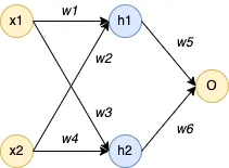
2.1. Network Structure

• 1 input layer (2 neurons)
• 1 hidden layer (2 neurons)
• 1 output layer (1 neuron)

2.2. Problem

• Input: \( [x_1, x_2] = [0.05, 0.10] \)
• Output: 0.01
• Learning Rate: 0.5

2.3. Random Initial Weights

• Weights between input and hidden layer: \( w_1 = 0.15, w_2 = 0.20, w_3 = 0.25, w_4 = 0.30 \)
• Weights between hidden and output layer: \( w_5 = 0.40, w_6 = 0.45 \)

2.4. Activation Function

• Sigmoid function: \( \sigma(x) = \frac{1}{1 + e^{-x}} \)

2.5. Forward Pass

2.5.1. Input to Hidden Layer

• Hidden Neuron 1:

\[ h_1 = \sigma(x_1 \cdot w_1 + x_2 \cdot w_2) = \sigma(0.05 \cdot 0.15 + 0.10 \cdot 0.20) = \sigma(0.0075 + 0.02) = \sigma(0.0275) = 0.5069 \]

• Hidden Neuron 2:

\[ h_2 = \sigma(x_1 \cdot w_3 + x_2 \cdot w_4) = \sigma(0.05 \cdot 0.25 + 0.10 \cdot 0.30) = \sigma(0.0125 + 0.03) = \sigma(0.0425) = 0.5106 \]

2.5.2. Hidden to Output Layer

\[ Output = \sigma(h_1 \cdot w_5 + h_2 \cdot w_6) = \sigma(0.5069 \cdot 0.40 + 0.5106 \cdot 0.45) = \sigma(0.2028 + 0.2298) = \sigma(0.4326) = 0.6069 \]

2.6. Error Calculation (Loss)

Use Mean Squared Error (MSE)

\[ E = \frac{1}{2} (t – o)^2 \]

• $\backslash (t\backslash )$ is the actual value.
• \(o\) is the output (predicted) value.

\[ E = \frac{1}{2}(t – o)^2 = \frac{1}{2}(0.01 – 0.6069)^2 = \frac{1}{2}(-0.5969)^2 = 0.178 \]

2.7. Backpropagation

2.7.1. Output to Hidden Layer

• Calculate gradient of the error with respect to the output:

\[  \frac{\partial E}{\partial o} = \frac{\partial}{\partial o} \left( \frac{1}{2} (t – o)^2 \right) \]

\[ \Rightarrow \frac{\partial E}{\partial o} = \frac{1}{2} \cdot \frac{\partial}{\partial o} \left( (t – o)^2 \right) \]

Apply the chain rule, we have

\[ \frac{\partial}{\partial o} \left( (t – o)^2 \right) = 2(t – o) \cdot \frac{\partial}{\partial o}(t – o) \]

Since \(t\) is a constant and does not depend on \(o\)

\[ \Rightarrow \frac{\partial E}{\partial o} = \frac{1}{2} \cdot 2(t – o) \cdot (-1) \]

\[ \Rightarrow \frac{\partial E}{\partial o} = o – t \]

\[ \Rightarrow \frac{\partial E}{\partial o} = o – t = 0.6069 – 0.01 = 0.5969 \]

• Calculate gradient of the output with respect to the net input (the derivative of Sigmoid function):

\[ \frac{\partial o}{\partial net_o} = o(1 – o) = 0.6069(1 – 0.6069) = 0.2384 \]

• Calculate total gradient for the output neuron:

\[ \delta_o = \frac{\partial E}{\partial net_o} = \frac{\partial E}{\partial o} \cdot \frac{\partial o}{\partial net_o} = 0.5969 \cdot 0.2384 = 0.1423 \]

• Adjust weights between hidden and output neurons (weights in neural network):

\[ \Delta w_5 = -\eta \cdot \delta_o \cdot h_1 = -0.5 \cdot 0.1423 \cdot 0.5069 = -0.036 \]

\[ \Delta w_6 = -\eta \cdot \delta_o \cdot h_2 = -0.5 \cdot 0.1423 \cdot 0.5106 = -0.0363 \]

• Update weights:

\[ w_5 = 0.40 – 0.036 = 0.364 \]

\[ w_6 = 0.45 – 0.0363 = 0.4137 \]

2.7.2. Hidden Layer to Input Layer

• Calculate the gradient for the hidden neurons:

\[ \frac{\partial E}{\partial net_{h1}} = \frac{\partial E}{\partial h1} \cdot \frac{\partial h1}{\partial net_{h1}} \]

\[ \Rightarrow \frac{\partial E}{\partial net_{h1}} = \frac{\partial E}{\partial net_o} \cdot \frac{\partial net_o}{\partial h1} \cdot \frac{\partial h1}{\partial net_{h1}} \]

\[ \Rightarrow \frac{\partial E}{\partial net_{h1}} = \delta_o \cdot \frac{\partial net_o}{\partial h1} \cdot h1(1-h1) \]

We have \(net_o = h_1w_5 + h_2w_6 \) so \( \frac{\partial net_o}{\partial h1} = w_5 \)

\[ \Rightarrow \delta_{h1} = \frac{\partial E}{\partial net_{h1}} = \delta_o \cdot w_5 \cdot h1(1-h1) \]

\[ \Rightarrow \delta_{h1} = 0.1423 \cdot 0.40 \cdot 0.5069(1 – 0.5069) = 0.0147 \]

Similarly we can calculate

\[ \delta_{h2} = \frac{\partial E}{\partial net_{h2}} = \delta_o \cdot w_6 \cdot h2(1-h2) \]

\[ \Rightarrow \delta_{h2} = 0.1423 \cdot 0.45 \cdot 0.5106(1 – 0.5106) = 0.0158 \]

• Adjust weights between input and hidden neurons:

\[ \Delta w_1 = -\eta \cdot \delta_{h1} \cdot x_1 = -0.5 \cdot 0.0147 \cdot 0.05 = -0.0004 \]

\[ \Delta w_2 = -\eta \cdot \delta_{h1} \cdot x_2 = -0.5 \cdot 0.0147 \cdot 0.10 = -0.0007 \]

\[ \Delta w_3 = -\eta \cdot \delta_{h2} \cdot x_1 = -0.5 \cdot 0.0158 \cdot 0.05 = -0.0004 \]

\[ \Delta w_4 = -\eta \cdot \delta_{h2} \cdot x_2 = -0.5 \cdot 0.0158 \cdot 0.10 = -0.0008 \]

• Update weights:

\[  w_1 = 0.15 – 0.0004 = 0.1496 \]

\[  w_2 = 0.20 – 0.0007 = 0.1993 \]

\[ w_3 = 0.25 – 0.0004 = 0.2496 \]

\[ w_4 = 0.30 – 0.0008 = 0.2992 \]

2.7.3. Repeat

This process is repeated for many iterations until the error becomes small enough, meaning the network has learned the relationship between inputs and outputs.