Linear Regression

Linear Regression is defined as an algorithm that provides a linear relationship between an independent variable and a dependent variable to predict the outcome of future events. It’s a basic algorithm of supervised learning.

For example, from the price dataset of more than 4000 houses, we will build a model to predict the house price that based on 3 attributes: bedrooms, bathrooms & floors. The input values are defined as a column vector:

$$
\mathbf{x} =
\begin{bmatrix}
x_1 \\
x_2 \\
x_3 \\
\end{bmatrix}
$$

So we have the output model that depends on the input values:

$$
\begin{align}
y \approx \hat{y} = f(x) &= x_1w_1 + x_2w_2 + x_3w_3 \\ &=
\begin{bmatrix}
x_1 & x_2 & x_3
\end{bmatrix}
\begin{bmatrix}
w_1 \\
w_2 \\
w_3 \\
\end{bmatrix} \\
&= \mathbf{x}^T\mathbf{w}
\end{align}
$$

Our expectation is that the prediction error \(e\) between \(y\) & \(\hat{y}\) should be minimum.

$$
\begin{align}
\frac{1}{2}e^2 = \frac{1}{2}(y-\hat{y})^2 = \frac{1}{2}(y-\mathbf{x}^T\mathbf{w})^2
\end{align}
$$

We have to use the square of \(e\) because \(y-\hat{y}\) can be negative. \(\frac{1}{2}\) is used to simplify the calculation of derivatives.

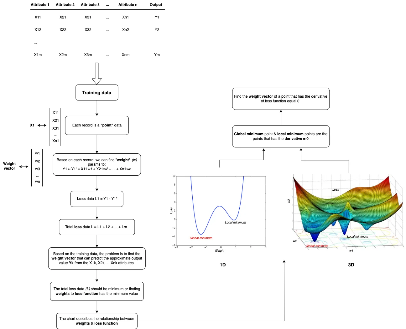
1. Loss function

When we have \(N\) training data points, each traning data point has the prediction error. Our problem is to create a model so that the sum of the prediction errors is minimum. It’s similar to find the weight vector \(\mathbf{w}\) so that the following function has the minimum value.

$$
\begin{align}
\mathcal{L}(\mathbf{w}) = \frac{1}{2N}\sum_{i=1}^N (y_i – \mathbf{x}_i^T\mathbf{w}_i)^2
\end{align}
$$

In machine learning, the loss function is the average of the error at each point that why we have the \(\frac{1}{2N}\) in that formula. As you can see, \(\mathcal{L}(\mathbf{w})\) has the relationship with 2-norm, so we can transform above formula to:

$$
\begin{align}
\mathcal{L}(\mathbf{w}) &= \frac{1}{2N} ||
\begin{bmatrix}
y_1 \\
y_2 \\
\vdots \\
y_N \\
\end{bmatrix} –
\begin{bmatrix}
\mathbf{x}_1^T \\
\mathbf{x}_2^T \\
\vdots \\
\mathbf{x}_N^T \\
\end{bmatrix} \mathbf{w}
||_2^2 \\
&= \frac{1}{2N} \|\mathbf{y} – \mathbf{X^T}\mathbf{w} \|_2^2
\end{align}
$$

2. Solution

The next step, we need to find the solution for that loss function by solving the derivative equation.

$$
\begin{align}
\mathcal{L}(\mathbf{w}) &= \frac{1}{2N} \|\mathbf{y} – \mathbf{X^T}\mathbf{w} \|_2^2 \\
&= \frac{1}{2N} (\mathbf{y} – \mathbf{X^T}\mathbf{w})^T(\mathbf{y} – \mathbf{X^T}\mathbf{w}) ~~~ (2.1)
\end{align}
$$

We have this transformation by using the equation \(||x||_2^2 = x^Tx\) when \(x\) is a vector. Let’s prove this one:

$$
\begin{align}
x =
\begin{bmatrix}
x_1 \\
x_2 \\
x_3
\end{bmatrix}
\Rightarrow x^Tx =
\begin{bmatrix}
x_1 & x_2 & x_3
\end{bmatrix}
\begin{bmatrix}
x_1 \\
x_2 \\
x_3
\end{bmatrix}
= x_1^2 + x_2^2 + x_3^2 = ||x||_2^2
\end{align}
$$

From (2.1) we have

$$
\begin{align}
\frac{\nabla \mathcal{L}(\mathbf{w})}{\nabla \mathbf{w}} &= \frac{1}{N}(\mathbf{X}\mathbf{X^T}\mathbf{w} – \mathbf{X}\mathbf{y}) ~~~ (2.2)
\end{align}
$$

You can read this post to understand about (2.2)

$$
\begin{align}
\frac{\nabla \mathcal{L}(\mathbf{w})}{\nabla \mathbf{w}} = 0 \iff \mathbf{X}\mathbf{X^T}\mathbf{w} = \mathbf{X}\mathbf{y}
\end{align} ~~~ (2.3)
$$

\(\mathbf{A} = \mathbf{X}\mathbf{X^T}\) is a square matrix.

– If \(\mathbf{A}\) is invertible, so (2.3) has the solution:

$$
\mathbf{w} = \mathbf{A}^{-1} \mathbf{X}\mathbf{y}
$$

– If \(\mathbf{A}\) is not invertible, we must find pseudoinverse \(\mathbf{A}^+\) of \(\mathbf{A}\). We know that every matrix has a SVD, so now the problem is to find pseudoinverse of a SVD.

$$
\begin{align}
\mathbf{w} &= \mathbf{A}^+ \mathbf{X}\mathbf{y} \\
&= (U \Sigma V^T)^+ \mathbf{X}\mathbf{y} \\
&= V \Sigma^+ U^T \mathbf{X}\mathbf{y}
\end{align} ~~~ (2.4)
$$

Where \(\Sigma^+\) is formed from \(\Sigma\) by taking the reciprocal of all the non-zero elements, leaving all the zeros alone, and making the matrix the right shape. If \(\Sigma\) is an \(m \times n\) matrix, then \(\Sigma^+\) must be an \(n \times m\) matrix.

In fact, solving derivative equations is an expensive calculation. So we need to use another way (Gradient Descent) to find the minimum of a function. It should be cheaper (faster) to find the solution using the gradient descent.