Linear Regression with PyTorch

1. Create training data

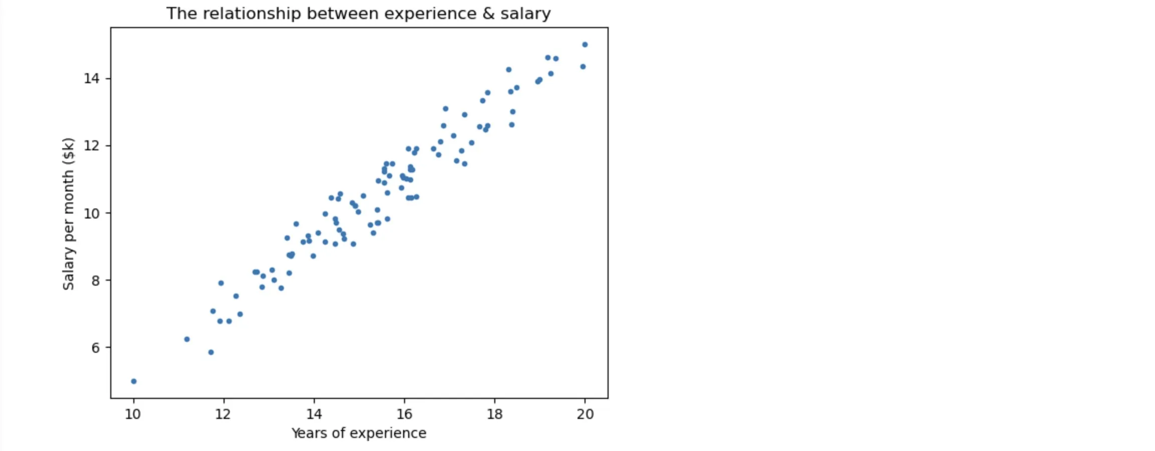
We’re going to use Scikit-learn package to generate the regression dataset between salary & experience with 100 samples & 1 feature

    from sklearn.datasets import make_regression
from sklearn.model_selection import train_test_split
import matplotlib.pyplot as plt 
import numpy as np 

x, y = make_regression(n_samples=100, n_features=1, noise=10, random_state=0)

x = np.interp(x, (x.min(), x.max()), (10, 20))
y = np.interp(y, (y.min(), y.max()), (5, 15))

plt.plot(x, y, '.')
plt.xlabel('Years of experience')
plt.ylabel('Salary per month ($k)')
plt.title('The relationship between experience & salary')
plt.show()

The next step, we will spit the dataset into 2 parts: 70% is used for training, 30% is used for testing

    xTrain, xTest, yTrain, yTest = train_test_split(x, y, test_size=0.3, random_state=0)

2. Build model

2.1. Linear model

The Linear Regression model:

https://pytorch.org/docs/stable/generated/torch.nn.Linear.html

    import torch
import torch.nn as nn

class LinearRegression(nn.Module):
    def __init__(self, input_dim, output_dim):
        super(LinearRegression, self).__init__()
        self.linear = nn.Linear(input_dim, output_dim)
        
    def forward(self, x):
        out = self.linear(x)
        return out

The input params of nn.Linear class are size of each input sample & output sample. Because we’ve chosen n_features = 1 so we have

    model = LinearRegression(1, 1)

2.2. Loss class

The next step, we will define the loss function. You can read more about the loss function in this post.

https://pytorch.org/docs/stable/generated/torch.nn.MSELoss.html

    criterion = nn.MSELoss()

2.3. Optimizer class

When the loss function is defined, we need to optimize the loss function to be the minimum value. The gradient descent algorithm is used in this case.

https://pytorch.org/docs/stable/generated/torch.optim.SGD.html

    learningRate = 0.1
optimizer = torch.optim.SGD(model.parameters(), lr=learningRate)

2.4. Train the model

In this section, we need to understand about “epoch”. What is “epoch”?

An epoch is when all the training data is used at once and we also need to defined “epochs” as the total number of iterations of all the training data in the machine learning model.

    losses = []
epochs = 100
for epoch in range(epochs):
    epoch += 1
    
    # Convert numpy array to torch
    inputs = torch.from_numpy(xTrain).to(torch.float32)
    labels = torch.from_numpy(yTrain).to(torch.float32)

    optimizer.zero_grad() 

    outputs = model(inputs)

    loss = criterion(outputs, labels)
    losses.append(loss.item())

    loss.backward()

    optimizer.step()

    print('Epoch: {} | Loss: {}'.format(epoch, loss.item()))

The output result:

    Epoch: 1 | Loss: 10.526817321777344
Epoch: 2 | Loss: 7.437290191650391
Epoch: 3 | Loss: 6.601305961608887
Epoch: 4 | Loss: 6.375033855438232
Epoch: 5 | Loss: 6.313724517822266
Epoch: 6 | Loss: 6.297047138214111
Epoch: 7 | Loss: 6.292445182800293
Epoch: 8 | Loss: 6.291110992431641
Epoch: 9 | Loss: 6.2906599044799805
Epoch: 10 | Loss: 6.290448188781738
Epoch: 11 | Loss: 6.290301322937012
Epoch: 12 | Loss: 6.2901716232299805
Epoch: 13 | Loss: 6.290046215057373
Epoch: 14 | Loss: 6.289923667907715
Epoch: 15 | Loss: 6.28980016708374
Epoch: 16 | Loss: 6.289676666259766
Epoch: 17 | Loss: 6.289554119110107
Epoch: 18 | Loss: 6.289431095123291
Epoch: 19 | Loss: 6.289308071136475
Epoch: 20 | Loss: 6.289185047149658
Epoch: 21 | Loss: 6.289062023162842
Epoch: 22 | Loss: 6.288939476013184
Epoch: 23 | Loss: 6.288815975189209
Epoch: 24 | Loss: 6.288693428039551
Epoch: 25 | Loss: 6.288570404052734
Epoch: 26 | Loss: 6.288447856903076
Epoch: 27 | Loss: 6.288325309753418
Epoch: 28 | Loss: 6.288203239440918
Epoch: 29 | Loss: 6.288079738616943
Epoch: 30 | Loss: 6.287956714630127
Epoch: 31 | Loss: 6.287834167480469
Epoch: 32 | Loss: 6.287710666656494
Epoch: 33 | Loss: 6.287587642669678
Epoch: 34 | Loss: 6.2874650955200195
Epoch: 35 | Loss: 6.2873430252075195
Epoch: 36 | Loss: 6.287219524383545
Epoch: 37 | Loss: 6.287096977233887
Epoch: 38 | Loss: 6.2869744300842285
Epoch: 39 | Loss: 6.286850452423096
Epoch: 40 | Loss: 6.286728858947754
Epoch: 41 | Loss: 6.2866058349609375
Epoch: 42 | Loss: 6.286482810974121
Epoch: 43 | Loss: 6.286359786987305
Epoch: 44 | Loss: 6.2862372398376465
Epoch: 45 | Loss: 6.286114692687988
Epoch: 46 | Loss: 6.285992622375488
Epoch: 47 | Loss: 6.285869598388672
Epoch: 48 | Loss: 6.2857465744018555
Epoch: 49 | Loss: 6.285624027252197
Epoch: 50 | Loss: 6.285501480102539
Epoch: 51 | Loss: 6.285378456115723
Epoch: 52 | Loss: 6.2852559089660645
Epoch: 53 | Loss: 6.2851338386535645
Epoch: 54 | Loss: 6.28501033782959
Epoch: 55 | Loss: 6.284887790679932
Epoch: 56 | Loss: 6.284765720367432
Epoch: 57 | Loss: 6.284642696380615
Epoch: 58 | Loss: 6.284520626068115
Epoch: 59 | Loss: 6.284398078918457
Epoch: 60 | Loss: 6.284275531768799
Epoch: 61 | Loss: 6.284153461456299
Epoch: 62 | Loss: 6.284030437469482
Epoch: 63 | Loss: 6.283907890319824
Epoch: 64 | Loss: 6.283784866333008
Epoch: 65 | Loss: 6.28366231918335
Epoch: 66 | Loss: 6.283539772033691
Epoch: 67 | Loss: 6.283417224884033
Epoch: 68 | Loss: 6.283294677734375
Epoch: 69 | Loss: 6.283172130584717
Epoch: 70 | Loss: 6.283050060272217
Epoch: 71 | Loss: 6.282927989959717
Epoch: 72 | Loss: 6.282805442810059
Epoch: 73 | Loss: 6.282681941986084
Epoch: 74 | Loss: 6.282560348510742
Epoch: 75 | Loss: 6.282438278198242
Epoch: 76 | Loss: 6.282314777374268
Epoch: 77 | Loss: 6.282193183898926
Epoch: 78 | Loss: 6.282069683074951
Epoch: 79 | Loss: 6.281947612762451
Epoch: 80 | Loss: 6.281824588775635
Epoch: 81 | Loss: 6.281702995300293
Epoch: 82 | Loss: 6.281580924987793
Epoch: 83 | Loss: 6.281458377838135
Epoch: 84 | Loss: 6.281336307525635
Epoch: 85 | Loss: 6.281213283538818
Epoch: 86 | Loss: 6.281091213226318
Epoch: 87 | Loss: 6.280969619750977
Epoch: 88 | Loss: 6.28084659576416
Epoch: 89 | Loss: 6.280724048614502
Epoch: 90 | Loss: 6.28060245513916
Epoch: 91 | Loss: 6.280479431152344
Epoch: 92 | Loss: 6.280357360839844
Epoch: 93 | Loss: 6.280235290527344
Epoch: 94 | Loss: 6.280112266540527
Epoch: 95 | Loss: 6.279990196228027
Epoch: 96 | Loss: 6.2798686027526855
Epoch: 97 | Loss: 6.279745578765869
Epoch: 98 | Loss: 6.279623508453369
Epoch: 99 | Loss: 6.279501438140869
Epoch: 100 | Loss: 6.279379367828369

The next step, we will visualize the loss data on the chart

    # Visualizing the loss data
plt.plot(range(epochs), losses)
plt.show()

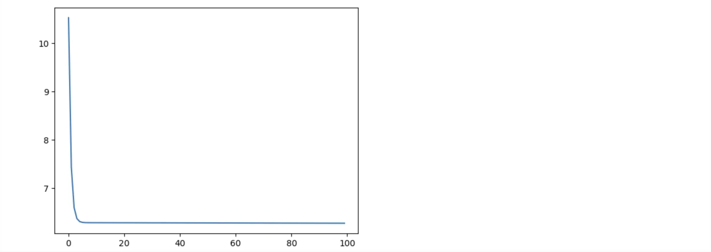
From the above result, we can see a considerable decrease in loss from epoch 1 to 3. From the 3rd epoch, the loss keeps almost steady. It means the model cannot further optimize itself.

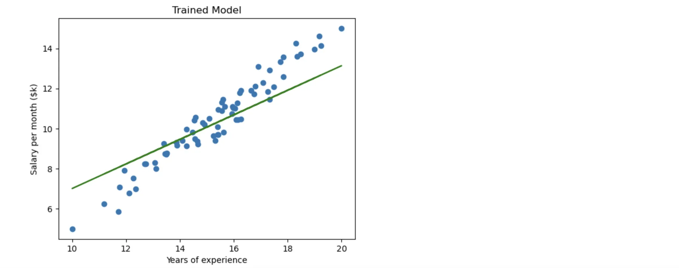
Let’s visualize the trained model:

    # Visualizing the trained model
def plotModel():
    plt.title('Trained Model')
    plt.xlabel('Years of experience')
    plt.ylabel('Salary per month ($k)')
    
    weight, bias = model.parameters()

    w = weight[0][0].item()
    b = bias[0].item()
    
    X1 = torch.from_numpy(xTrain).to(torch.float32)
    Y1 = w * X1 + b
    
    plt.plot(X1, Y1, 'g')
    plt.scatter(xTrain, yTrain)
    plt.show()

plotModel()

Here is the full source code:

    from sklearn.datasets import make_regression
from sklearn.model_selection import train_test_split
import matplotlib.pyplot as plt 
import numpy as np
import torch
import torch.nn as nn

x, y = make_regression(n_samples=100, n_features=1, noise=10, random_state=0)

x_train, x_test, y_train, y_test = train_test_split(x, y, test_size=0.33, random_state=42)

x = np.interp(x, (x.min(), x.max()), (10, 20))
y = np.interp(y, (y.min(), y.max()), (5, 15))

plt.plot(x, y, '.')
plt.xlabel('Years of experience')
plt.ylabel('Salary per month ($k)')
plt.title('The relationship between experience & salary')
plt.show()

xTrain, xTest, yTrain, yTest = train_test_split(x, y, test_size=0.3, random_state=0)

class LinearRegression(nn.Module):
    def __init__(self, input_dim, output_dim):
        super(LinearRegression, self).__init__()
        self.linear = nn.Linear(input_dim, output_dim)
        
    def forward(self, x):
        out = self.linear(x)
        return out

model = LinearRegression(1, 1)

criterion = nn.MSELoss()

learningRate = 0.001
optimizer = torch.optim.SGD(model.parameters(), lr=learningRate)

losses = []
epochs = 100
for epoch in range(epochs):
    epoch += 1
    
    # Convert numpy array to torch
    inputs = torch.from_numpy(xTrain).to(torch.float32)
    labels = torch.from_numpy(yTrain).to(torch.float32)

    optimizer.zero_grad() 

    outputs = model(inputs)

    loss = criterion(outputs, labels)
    losses.append(loss.item())

    loss.backward()

    optimizer.step()

    print('Epoch: {} | Loss: {}'.format(epoch, loss.item()))

# Visualizing the loss data
plt.plot(range(epochs), losses)
plt.show()

# Visualizing the trained model
def plotModel():
    plt.title('Trained Model')
    plt.xlabel('Years of experience')
    plt.ylabel('Salary per month ($k)')
    
    weight, bias = model.parameters()

    w = weight[0][0].item()
    b = bias[0].item()
    
    X1 = torch.from_numpy(xTrain).to(torch.float32)
    Y1 = w * X1 + b
    
    plt.plot(X1, Y1, 'g')
    plt.scatter(xTrain, yTrain)
    plt.show()

plotModel()