Long Short-Term Memory (LSTM)

LSTM (Long Short-Term Memory) is a type of Recurrent Neural Network (RNN) architecture designed to effectively learn and process sequences of data, such as time-series data, text, speech, and video. LSTM are designed to address the limitations of standard RNN, particularly the challenge of learning long-term dependencies in sequential data.

The main components of LSTM:

• Memory cells: LSTM have memory cells that store information for long periods, allowing the network to remember context over time.
• Forget gate: Decides what information to discard from the cell state.
• Input gate: Determines what new information to store in the cell state.
• Output gate: Controls what information to output from the cell state.
• Cell State: A direct way that allows information to pass through.

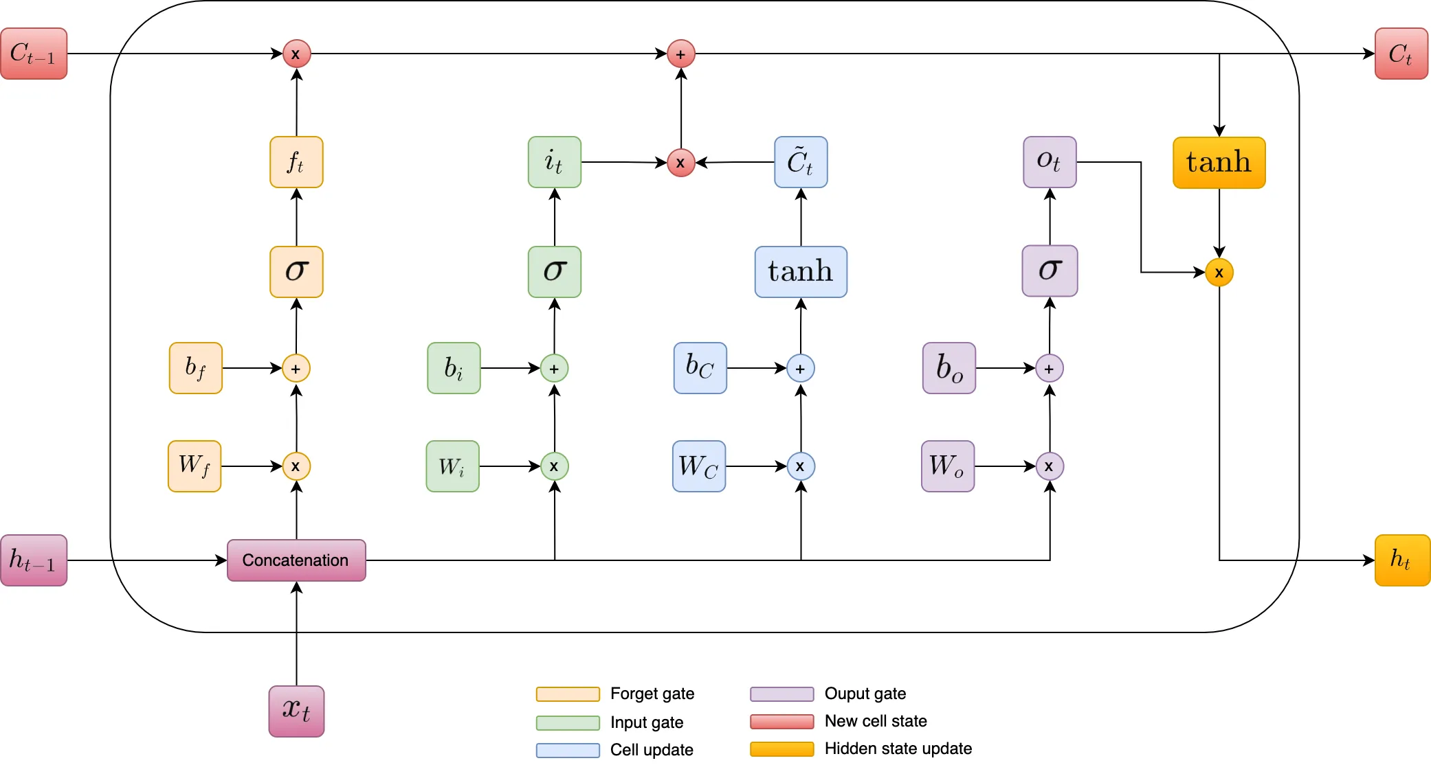
1. Forward Pass

1.1. Forget Gate

Forget Gate controls what old information should be removed from the memory. It helps the model focus on relevant information while discarding unnecessary or outdated data.

E.g. Predicting Bitcoin’s next price movement:

– Important: When whales (large holders) move BTC to or from exchanges, it can signal future price movements.

– Unimportant: A random crypto influencer tweets.

\[ f_t = \sigma(W_f \cdot [h_{t-1}, x_t] + b_f) ~~~~~~~~~~ (1.1) \]

• \(f_t\): The forget gate activation vector at time step \(t\). Each value in \(f_t\) is between 0 (forget the information) and 1 (keep the information).
• \(\sigma\): The sigmoid activation function. It ensures the output values are between 0 and 1.
• \(W_f \): The weight matrix for the forget gate.
• \(h_{t-1}\): The hidden state from the previous time step.
• \(x_t\): The input vector at the current time step.
• \(b_f\): The forget gate bias.

1.1.1. The concatenated vector

Given two vectors:

• \(h_{t-1}\): Hidden state from the previous time step (n-dimensional).
• \(x_t\): Input vector at the current time step (m-dimensional).

The concatenated vector \([h_{t-1}, x_t]\) is a new vector of size n + m. E.g.

\[ h_{t-1} = \begin{bmatrix} 0.5 \\ 0.3 \\ 0.8 \end{bmatrix}, \quad x_t = \begin{bmatrix} 0.9 \\ 0.4 \end{bmatrix} \]

\[ [h_{t-1}, x_t] = \begin{bmatrix} 0.5 \\ 0.3 \\ 0.8 \\ 0.9 \\ 0.4 \end{bmatrix} \]

1.2. Input Gate

Input Gate controls what new information should be added to the memory. It decides what new data is important and should be stored for future use.

E.g. Predicting Bitcoin’s next price movement:

– Important: A major exchange announces bankruptcy, the event should be added to memory because it could lead to a price crash.

– Unimportant: If small daily price fluctuations occur, the input gate might block it from entering memory.

\[  i_t = \sigma(W_i \cdot [h_{t-1}, x_t] + b_i) ~~~~~~~~~~ (1.2) \]

• \(i_t\): The input gate activation vector at time step \(t\), with values between 0 and 1.
• \(\sigma\): The sigmoid activation function. It ensures the output values are between 0 and 1.
• \(W_i\): The weight matrix for the input gate.
• \(h_{t-1}\): The hidden state from the previous time step.
• \(x_t\): The input vector at the current time step.
• \(b_i\): The bias vector for the input gate.

1.3. Cell Update

Cell update modifies the memory by combining both old and new information. It ensures the model retains relevant past knowledge while incorporating useful new data for better decision making.

E.g. Predicting Bitcoin’s next price movement:

– New important information: A major exchange announces bankruptcy.

– Outdated or irrelevant information: An old bullish trend from three weeks ago that is no longer influencing the market.

– The updated memory now reflects a higher probability of a BTC price drop due to negative market sentiment.

\[ \tilde{C}_t = \tanh(W_C \cdot [h_{t-1}, x_t] + b_C) ~~~~~~~~~~ (1.3) \]

• \(\tilde{C}_t\): It’s a potential update to the cell state at time step \(t\).
• \(\tanh\): The tanh activation function. It ensures the values in the range [-1, 1].
• \(W_C\): The weight matrix for the cell state.
• \(h_{t-1}\): The hidden state from the previous time step.
• \(x_t\): The input vector at the current time step.
• \(b_C\): The bias vector for the cell state.

1.4. Output Gate

Output Gate controls what part of the updated memory (cell state) should be used as the final output at the current time step. It decides how much of the stored information influences the next step in prediction.

E.g. Predicting Bitcoin’s next price movement:

– If the model needs to predict the next hour’s Bitcoin price, the output gate might reduce the influence of long term bullish trends.

– If predicting Bitcoin’s price for the next six months, the output gate may allow more long term memory to be used, such as institutional accumulation and historical bull/bear market cycles.

\[ o_t = \sigma(W_o \cdot [h_{t-1}, x_t] + b_o) ~~~~~~~~~~ (1.4) \]

• \(o_t\): The output gate activation vector at time step \(t\), with values between 0 and 1.
• \(\sigma\): The sigmoid activation function, which ensures values lie in the range [0,1].
• \(W_o\): The weight matrix for the output gate.
• \(h_{t-1}\): The hidden state from the previous time step.
• \(x_t\): The input vector at the current time step.
• \(b_o\): The bias vector for the output gate.

1.5. New Cell State

New Cell State acts as the updated memory that carries long term information forward while ensuring the model remains adaptable to new data.

\[ C_t = f_t \cdot C_{t-1} + i_t \cdot \tilde{C}_t  ~~~~~~~~~~ (1.5) \]

• \(C_t\): The new cell state at time step \(t\).
• \(C_{t-1}\): The previous cell state at time step \(t – 1\).
• \(f_t\): The forget gate activation.
• \(i_t\): The input gate activation.
• \(\tilde{C}_t\): It’s a potential update to the cell state at time step \(t\).

1.6. Hidden State Update

Hidden State represents the short term memory and serves as the immediate output of an LSTM at each time step.

\[ h_t = o_t \cdot \tanh(C_t) ~~~~~~~~~~ (1.6) \]

• \(h_t\): The hidden state at time step \(t\)$.$
• \(o_t\): The output gate activation.
• \(C_t\): The updated cell state at time step \(t\).

2. Loss

2.1. Output

In an LSTM network, the output (\(y_t\)) is not directly part of the cell state (\(C_t\)). Instead, it is derived from the hidden state (\(h_t\)). The common output activation functions:

• Softmax: For multi-class classification tasks.

\[ y_t = \text{Softmax}(W_y \cdot h_t + b_y) \]

• Sigmoid: For binary classification or probability estimation.

\[ y_t = \sigma(W_y \cdot h_t + b_y) \]

• Linear: For regression tasks or continuous output.

\[ y_t = W_y \cdot h_t + b_y \]

2.2. Loss at a single timestep

2.2.1. Mean Squared Error (MSE).

\[ \ell(y_t, \hat{y}_t) = (y_t – \hat{y}_t)^2 \]

• \({y}_t\): The true value at timestep \(t\).
• \(\hat{y}_t\): The predicted value at timestep \(t\).

2.2.2. Cross-Entropy Loss (for multi-class classification).

\[ \ell(y_t, \hat{y}_t) = – \sum_{c=1}^C y_t^c \log(\hat{y}_t^c) \]

• \(C\): Number of classes.
• \(y_t^c \): True label for class \(c\) at timestep \(t\).
• \(\hat{y}_t^c \): Predicted probability for class \(c\) at timestep \(t\).

3. Backward Pass (BPTT)

For the backward pass, the goal is to compute the gradients of the loss \(L\) with respect to all the parameters (weights, biases) at every time step \(t\) using the chain rule.

3.1. Gradient of Loss with respect to Hidden State

\[ \frac{\partial L}{\partial h_t} = \frac{\partial L}{\partial y_t} \cdot \frac{\partial y_t}{\partial h_t} \]

Based on (1.6) we need to compute:

3.1.1. Derivative of \(h_t\) respect to \(C_t\)

Because \(o_t\) is independent of \(C_t\)

\[ \frac{\partial h_t}{\partial C_t} = o_t \cdot \frac{\partial}{\partial C_t} \tanh(C_t) \]

See the derivative of tanh function

\[ \Rightarrow \frac{\partial h_t}{\partial C_t} = o_t \cdot (1 – \tanh^2(C_t)) ~~~~~~~~~~ (3.1.1) \]

3.1.2. Derivative of \(h_t\) respect to \(o_t\)

\[ \frac{\partial h_t}{\partial o_t} = \tanh(C_t) ~~~~~~~~~~ (3.1.2) \]

3.2. Gradient of Loss with respect to New Cell State

\[ \frac{\partial L}{\partial C_t} = \frac{\partial L}{\partial h_t} \cdot \frac{\partial h_t}{\partial C_t} \]

From (3.1.1)

\[ \Rightarrow \frac{\partial L}{\partial C_t} = \frac{\partial L}{\partial h_t} \cdot o_t \cdot (1 – \tanh^2(C_t)) \]

3.2.1. Derivative of Loss with respect to \(C_{t-1}\)

Based on (1.5) we have \(i_t\) & \(\tilde{C}_t\) do not depend on \(C_{t-1}\)

\[ \Rightarrow \frac{\partial C_t}{\partial C_{t-1}} = f_t \cdot \frac{\partial C_{t-1}}{\partial C_{t-1}} \]

\[ \Rightarrow \frac{\partial C_t}{\partial C_{t-1}} = f_t \]

Using the chain rule, we have:

\[ \frac{\partial L}{\partial C_{t-1}} = \frac{\partial L}{\partial C_t} \cdot \frac{\partial C_t}{\partial C_{t-1}} \]

\[ \Rightarrow \frac{\partial L}{\partial C_{t-1}} = \frac{\partial L}{\partial C_t} \cdot f_t ~~~~~~~~~~ (3.2.1) \]

3.2.2. Derivative of Loss with respect to \(f_t\)

Based on (1.5) we have:

\[ \frac{\partial C_t}{\partial f_t} = C_{t-1} \]

Using the chain rule, we have:

\[ \frac{\partial L}{\partial f_t} = \frac{\partial L}{\partial C_t} \cdot \frac{\partial C_t}{\partial f_t} \]

\[ \Rightarrow \frac{\partial L}{\partial f_t} = \frac{\partial L}{\partial C_t} \cdot C_{t-1} ~~~~~~~~~~ (3.2.2) \]

3.2.3. Derivative of Loss with respect to \(i_t\)

Based on (1.5) we have:

\[ \frac{\partial C_t}{\partial i_t} = \tilde{C_t} \]

Using the chain rule, we have:

\[ \frac{\partial L}{\partial i_t} = \frac{\partial L}{\partial C_t} \cdot \frac{\partial C_t}{\partial i_t} \]

\[ \Rightarrow \frac{\partial L}{\partial f_t} = \frac{\partial L}{\partial C_t} \cdot \tilde{C_t}  ~~~~~~~~~~ (3.2.3) \]

3.2.4. Derivative of Loss with respect to \(\tilde{C_t}\)

Based on (1.5) we have:

\[ \frac{\partial C_t}{\partial \tilde{C_t}} = i_t \]

Using the chain rule, we have:

\[ \frac{\partial L}{\partial \tilde{C_t}} = \frac{\partial L}{\partial C_t} \cdot \frac{\partial C_t}{\partial \tilde{C_t}} \]

\[ \Rightarrow \frac{\partial L}{\partial \tilde{C_t}} = \frac{\partial L}{\partial C_t} \cdot i_t  ~~~~~~~~~~ (3.2.4) \]

3.3. Gradient of Loss with respect to Output

\[ \frac{\partial L}{\partial o_t} = \frac{\partial L}{\partial h_t} \cdot \frac{\partial h_t}{\partial o_t} \]

Based on (1.6) we have

\[ \Rightarrow \frac{\partial L}{\partial o_t} = \frac{\partial L}{\partial h_t} \cdot \tanh(C_t) \]

Let see derivative of \(o_t\) with respect to \(W_o\). From (1.4) \(o_t\) is computed by using the sigmoid function. You can find the derivative of sigmoid function at here.

\[ z_o = W_o \cdot [h_{t-1}, x_t] + b_o \]

\[ \Rightarrow o_t = \sigma(z_o) \]

\[ \Rightarrow \frac{\partial o_t}{\partial W_o} = \frac{\partial \sigma(z_o)}{\partial z_o} \cdot \frac{\partial z_o}{\partial W_o} \]

\[ \Rightarrow \frac{\partial o_t}{\partial W_o} = o_t \cdot (1 – o_t) \cdot \frac{\partial z_o}{\partial W_o} \]

\[ \Rightarrow \frac{\partial o_t}{\partial W_o} = o_t \cdot (1 – o_t) \cdot [h_{t-1}, x_t] \]

\[ \Rightarrow \frac{\partial L}{\partial W_o} = \frac{\partial L}{\partial o_t} \cdot o_t \cdot (1 – o_t) \cdot [h_{t-1}, x_t] \]

3.4. Gradient of Loss with respect to Cell Update

\[ \frac{\partial L}{\partial \tilde{C}_t} = \frac{\partial L}{\partial C_t} \cdot \frac{\partial C_t}{\partial \tilde{C}_t} \]

Based on (1.5), we have:

\[ \frac{\partial C_t}{\partial \tilde{C}_t} = i_t \]

\[ \Rightarrow \frac{\partial L}{\partial \tilde{C}_t} = \frac{\partial L}{\partial C_t} \cdot i_t \]

Let see derivative of \(\tilde{C}_t\) with respect to \(W_C\). From (1.3) \(\tilde{C}_t\) is computed by using the tanh function. You can find the derivative of tanh function at here.

\[ z_C = W_C \cdot [h_{t-1}, x_t] + b_C \]

\[ \Rightarrow \tilde{C}_t = \tanh(z_C ) \]

Using the chain rule, we have:

\[ \Rightarrow \frac{\partial \tilde{C}_t}{\partial W_C} = \frac{\partial \tilde{C}_t}{\partial z_C} \cdot \frac{\partial z_C}{\partial W_C} \]

\[ \Rightarrow \frac{\partial \tilde{C}_t}{\partial W_C} = (1 – \tilde{C}_t^2) \cdot  [h_{t-1}, x_t] \]

\[ \Rightarrow \frac{\partial L}{\partial W_C} = \frac{\partial L}{\partial \tilde{C}_t} \cdot (1 – \tilde{C}_t^2) \cdot  [h_{t-1}, x_t] \]

3.5. Gradient of Loss with respect to Input Gate

\[ \frac{\partial L}{\partial i_t} = \frac{\partial L}{\partial C_t} \cdot \frac{\partial C_t}{\partial i_t} \]

Based on (1.5), we have:

\[ \frac{\partial C_t}{\partial i_t} = \tilde{C}_t \]

\[ \Rightarrow \frac{\partial L}{\partial i_t} = \frac{\partial L}{\partial C_t} \cdot \tilde{C}_t \]

Let see derivative of \(i_t\) with respect to \(W_i\). From (1.2) \(i_t\) is computed by using the sigmoid function. You can find the derivative of sigmoid function at here.

\[ z_i = W_i \cdot [h_{t-1}, x_t] + b_i \]

\[ \Rightarrow i_t = \sigma(z_i) \]

Using the chain rule, we have:

\[ \Rightarrow \frac{\partial i_t}{\partial W_i} = \frac{\partial i_t}{\partial z_i} \cdot \frac{\partial z_i}{\partial W_i} \]

\[ \Rightarrow \frac{\partial i_t}{\partial W_i} = i_t \cdot (1 – i_t) \cdot [h_{t-1}, x_t] \]

\[ \Rightarrow \frac{\partial L}{\partial W_i} = \frac{\partial L}{\partial i_t} \cdot i_t \cdot (1 – i_t) \cdot [h_{t-1}, x_t] \]

3.6. Gradient of Loss with respect to Forget Gate

\[ \frac{\partial L}{\partial f_t} = \frac{\partial L}{\partial C_t} \cdot \frac{\partial C_t}{\partial f_t} \]

Based on (1.5), we have:

\[ \frac{\partial C_t}{\partial f_t} = C_{t-1} \]

\[ \Rightarrow \frac{\partial L}{\partial f_t} = \frac{\partial L}{\partial C_t} \cdot C_{t-1} \]

Let see derivative of \(f_t\) with respect to \(W_f\). From (1.1) \(f_t\) is computed by using the sigmoid function. You can find the derivative of sigmoid function at here.

\[ z_f = W_f \cdot [h_{t-1}, x_t] + b_f \]

\[ \Rightarrow f_t = \sigma(z_f) \]

Using the chain rule, we have:

\[ \Rightarrow \frac{\partial f_t}{\partial W_f} = \frac{\partial f_t}{\partial z_f} \cdot \frac{\partial z_f}{\partial W_f} \]

\[ \Rightarrow \frac{\partial f_t}{\partial W_f} = f_t \cdot (1 – f_t) \cdot [h_{t-1}, x_t] \]

\[ \Rightarrow \frac{\partial L}{\partial W_f} = \frac{\partial L}{\partial f_t} \cdot f_t \cdot (1 – f_t) \cdot [h_{t-1}, x_t]  \]

4. Optimization

The result from BPTT step:

\[ \frac{\partial L}{\partial W_o} = \frac{\partial L}{\partial o_t} \cdot o_t \cdot (1 – o_t) \cdot [h_{t-1}, x_t] \]

\[ \frac{\partial L}{\partial W_C} = \frac{\partial L}{\partial \tilde{C}_t} \cdot (1 – \tilde{C}_t^2) \cdot  [h_{t-1}, x_t] \]

\[ \frac{\partial L}{\partial W_i} = \frac{\partial L}{\partial i_t} \cdot i_t \cdot (1 – i_t) \cdot [h_{t-1}, x_t] \]

\[ \frac{\partial L}{\partial W_f} = \frac{\partial L}{\partial f_t} \cdot f_t \cdot (1 – f_t) \cdot [h_{t-1}, x_t]  \]

These gate activations \(o_t, \tilde{C}_t, i_t, f_t\) are intermediate variables inside the LSTM cell. Since the loss \(L\) does not directly depend on these gates but rather on \(h_t, C_t\). So we need to express above formulas​ in terms of computable values.

4.1. Derivative of Loss with respect to \(W_o\)

\[ \frac{\partial L}{\partial W_o} = \frac{\partial L}{\partial o_t} \cdot o_t \cdot (1 – o_t) \cdot [h_{t-1}, x_t] \]

Based on (1.6) we have

\[ \frac{\partial L}{\partial o_t} = \frac{\partial L}{\partial h_t} \cdot \tanh(C_t) \]

\[ \Rightarrow \frac{\partial L}{\partial W_o} = \frac{\partial L}{\partial h_t} \cdot \tanh(C_t) \cdot o_t \cdot (1 – o_t) \cdot [h_{t-1}, x_t] \]

4.2. Derivative of Loss with respect to \(W_C\)

\[ \frac{\partial L}{\partial W_C} = \frac{\partial L}{\partial \tilde{C}_t} \cdot (1 – \tilde{C}_t^2) \cdot  [h_{t-1}, x_t] \]

Based on (1.5) we have

\[ \frac{\partial C_t}{\partial \tilde{C}_t} = i_t \]

\[ \Rightarrow \frac{\partial L}{\partial \tilde{C}_t} = \frac{\partial L}{\partial C_t} \cdot i_t \]

\[ \Rightarrow \frac{\partial L}{\partial W_C} = \frac{\partial L}{\partial C_t} \cdot i_t \cdot (1 – \tilde{C}_t^2) \cdot  [h_{t-1}, x_t] \]

4.3. Derivative of Loss with respect to \(W_i\)

\[ \frac{\partial L}{\partial W_i} = \frac{\partial L}{\partial i_t} \cdot i_t \cdot (1 – i_t) \cdot [h_{t-1}, x_t] \]

Based on (1.5) we have

\[ \frac{\partial C_t}{\partial i_t} = \tilde{C}_t \]

\[ \Rightarrow \frac{\partial L}{\partial i_t} = \frac{\partial L}{\partial C_t} \cdot \tilde{C}_t \]

\[ \Rightarrow \frac{\partial L}{\partial W_i} = \frac{\partial L}{\partial C_t} \cdot \tilde{C}_t \cdot i_t \cdot (1 – i_t) \cdot [h_{t-1}, x_t] \]

4.3. Derivative of Loss with respect to \(W_f\)

\[ \frac{\partial L}{\partial W_f} = \frac{\partial L}{\partial f_t} \cdot f_t \cdot (1 – f_t) \cdot [h_{t-1}, x_t]  \]

Based on (1.5) we have

\[ \frac{\partial C_t}{\partial f_t} = C_{t-1} \]

\[ \Rightarrow \frac{\partial L}{\partial f_t} = \frac{\partial L}{\partial C_t} \cdot C_{t-1} \]

\[ \Rightarrow \frac{\partial L}{\partial W_f} = \frac{\partial L}{\partial C_t} \cdot C_{t-1} \cdot f_t \cdot (1 – f_t) \cdot [h_{t-1}, x_t]  \]

– Unlike feedforward networks where each layer has a unique set of weights, LSTM reuses the same weight matrices at every time step. The four main LSTM weights \( W_o, W_C, W_i, W_f \) are shared across all time steps.

– At each time step \(t\), the forward pass computes \( f_t, i_t, \tilde{C}_t, o_t, C_t, h_t \). After processing all time steps, we apply BPTT to accumulate gradients over all time steps before updating the weights.

Since the same weights are used at every time step, the total gradient for each weight matrix is:

\[ \frac{\partial L}{\partial W} = \sum_{t=1}^{T} \frac{\partial L_t}{\partial W} \]

• \( T \) is the total number of time steps.
• \( \frac{\partial L_t}{\partial W} \) is the gradient computed at time step \(t\).

4.4. Weight update formulas

\[ W_f^{\text{new}} = W_f^{\text{old}} – \eta \sum_{t=1}^{T} \frac{\partial L_t}{\partial W_f} \]

\[ W_i^{\text{new}} = W_i^{\text{old}} – \eta \sum_{t=1}^{T} \frac{\partial L_t}{\partial W_i} \]

\[ W_C^{\text{new}} = W_C^{\text{old}} – \eta \sum_{t=1}^{T} \frac{\partial L_t}{\partial W_C} \]

\[ W_o^{\text{new}} = W_o^{\text{old}} – \eta \sum_{t=1}^{T} \frac{\partial L_t}{\partial W_o} \]

Read more about Gradient Descent

References:

• https://web.stanford.edu/class/cs379c/archive/2018/class_messages_listing/content/Artificial_Neural_Network_Technology_Tutorials/OlahLSTM-NEURAL-NETWORK-TUTORIAL-15.pdf
• https://gdac.uqam.ca/Workshop@EDM20/slides/LSTM_Tutorial.pdf