Probability Distributions

In probability and statistics, there are many types of distributions, each suited for different types of data and analysis. They can be categorized into discrete and continuous distributions.

1. Discrete Distributions

Discrete distributions are probability distributions that describe phenomena with countable outcomes. These outcomes can be finite or countably infinite, and the probability of each outcome can be explicitly stated. They are particularly useful in scenarios where the data or events are distinct and separate. (Eg. rolling a fair six-sided die)

1.1. Characteristics of Discrete Distributions

– The random variable can take on a finite or countably infinite number of distinct values.

\[ X \in \{x_1, x_2, x_3, \ldots, x_n\} \]

– The probability of each outcome is described by a PMF (Probability Mass Function).

\[ P(X = x_i) = p_i \quad \text{for } i = 1, 2, \ldots, n \]

– Each probability value is non-negative and lies between 0 and 1.

\[ 0 \leq P(X = x_i) \leq 1 \]

– The sum of the probabilities for all possible outcomes is equal to 1.

\[ \sum_{i=1}^{n} P(X = x_i) = 1 \]

1.2. Expected Value

The expected value of a discrete random variable is a measure of the center of its distribution. For a discrete random variable \( X \) with possible values \( x_1, x_2, \ldots, x_n \) is

\[ E(X) = \sum_{i=1}^{n} x_i P(X = x_i) \]

Eg. We have a discrete random variable \(X\) that represents the outcome of rolling a fair six-sided die. The possible values of \(X\) are 1, 2, 3, 4, 5, and 6, each with an equal probability of 1/6.

\[ E(X) = 1 \cdot \frac{1}{6} + 2 \cdot \frac{1}{6} + 3 \cdot \frac{1}{6} + 4 \cdot \frac{1}{6} + 5 \cdot \frac{1}{6} + 6 \cdot \frac{1}{6} \]

\[ \Rightarrow E(X) = 3.5 \]

It means that if you repeatedly roll a fair six-sided die, the average value of the outcomes will approach the expected value (3.5) over a large number of rolls.

1.3. Variance

Variance is a measure of the spread or dispersion of a set of values. It quantifies how much the values of the random variable differ from the expected value.

\[ \text{Var}(X) = \sum_{i=1}^n (x_i – E(X))^2 P(X = x_i) \]

We square the differences when calculating the variance to ensure all deviations from the mean are non-negative and to give greater weight to larger deviations. From above rolling a fair six-sided die example, we have:

\[ \text{Var}(X) = \sum_{i=1}^6 (x_i – 3.5)^2 P(X = x_i) \]

\[ \Rightarrow \text{Var}(X) = \frac{1}{6} \left[ (1 – 3.5)^2 + (2 – 3.5)^2 + (3 – 3.5)^2 + (4 – 3.5)^2 + (5 – 3.5)^2 + (6 – 3.5)^2 \right] \]

\[ \Rightarrow \text{Var}(X) = \frac{1}{6} \left[ 6.25 + 2.25 + 0.25 + 0.25 + 2.25 + 6.25 \right] = \frac{17.5}{6} \approx 2.9167 \]

1.4. Some main types of Discrete Distribution

• Binomial Distribution
• Poisson Distribution
• Geometric Distribution
• Negative Binomial Distribution
• Hypergeometric Distribution
• Uniform Distribution
• Bernoulli Distribution

2. Continuous Distributions

Continuous distributions are probability distributions that deal with continuous random variables. A continuous random variable can take any value within a specified range (which can be finite or infinite). Unlike discrete distributions, which are defined at specific points, continuous distributions are defined over an interval or range of values.

2.1. Probability Density Function (PDF)

A Probability Density Function (PDF) is a fundamental concept in continuous probability distributions. It describes the likelihood of a continuous random variable taking on a particular value.

– The PDF \(f(x)\) must be non-negative for all possible values of \(x\)

\[ f(x) \geq 0 \quad \]

– The integral of the PDF over the entire range of the random variable must equal 1

\[ \int_{-\infty}^{\infty} f(x) \, dx = 1 \]

– The probability that a continuous random variable \(X\) lies within a specific interval \([a,b]\) is given by the integral of the PDF over that interval

\[ P(a \leq X \leq b) = \int_{a}^{b} f(x) \, dx \]

There are several common types of PDF, each associated with a specific continuous probability distribution. Here are some of the most common types:

• Normal Distribution
• Uniform Distribution
• Exponential Distribution
• Log-Normal Distribution
• Beta Distribution
• Gamma Distribution
• Weibull Distribution
• Chi-Square Distribution

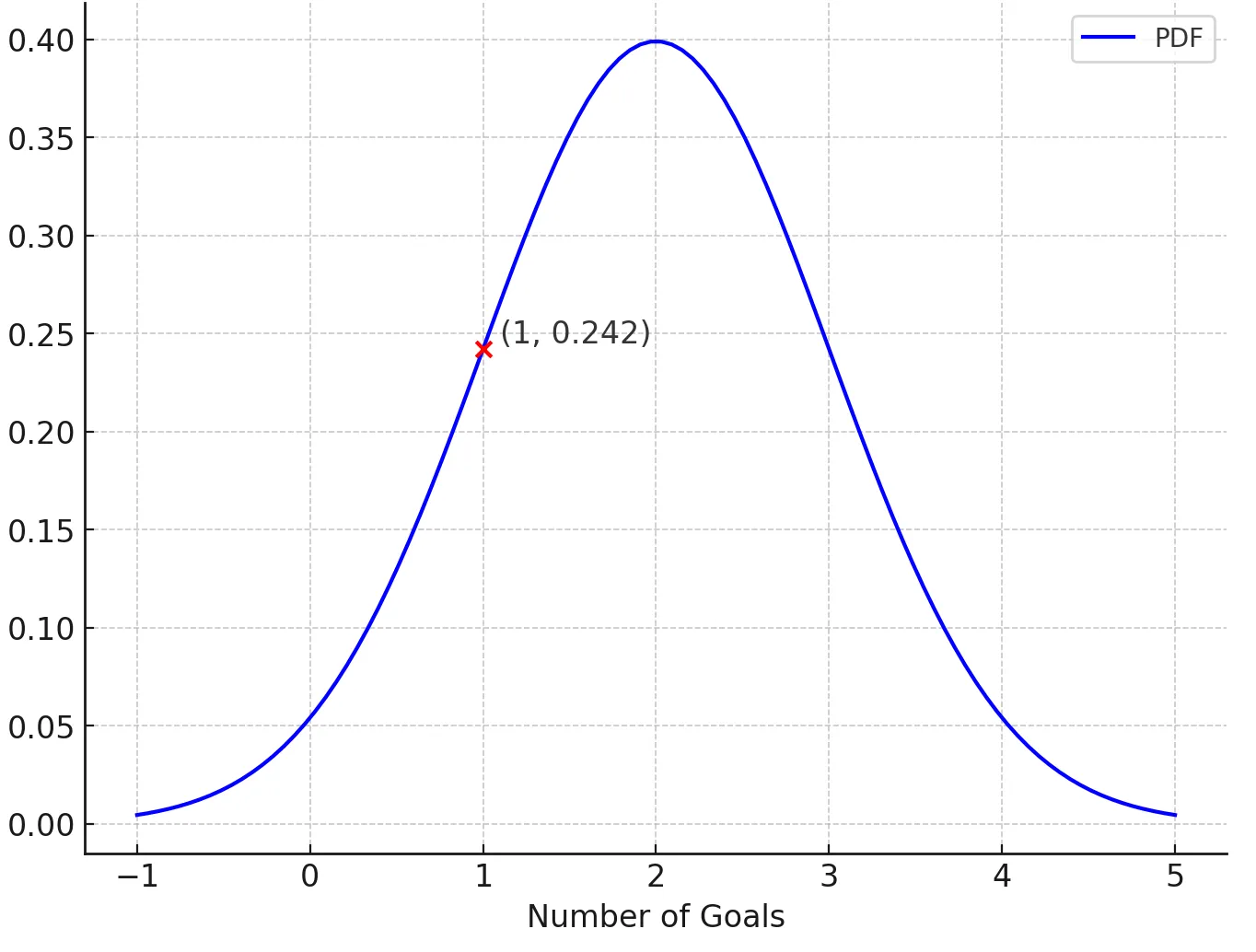
The most well-known type of PDF is the Normal Distribution. The formula is:

\[ f(x) = \frac{1}{\sigma \sqrt{2\pi}} e^{-\frac{1}{2}\left(\frac{x-\mu}{\sigma}\right)^2} ~~~~~~~~~ (2.1.1) \]

• \(\mu\) is the mean of the distribution.
• $\backslash (\backslash sigma\backslash )$ is the standard deviation.
• $\backslash (x\backslash )$ is the variable of interest.

Let’s see a basic example. You are analyzing the performance of a football team and want to understand how often they score a certain number of goals in a game. You know that:

• The average number of goals scored by the team per game (\(\mu\)) is 2.
• The standard deviation ($\backslash (\backslash sigma\backslash )$) of goals per game is 1.

The question: What is the probability density of the team scoring exactly 1 \((x)\) goal in a game?

From (2.1.1) formula, we have:

\[ f(1|2, 1^2) = \frac{1}{\sqrt{2\pi(1)^2}} e^{-\frac{(1-2)^2}{2(1)^2}} \]

\[ \Rightarrow f(1|2, 1^2) = \frac{1}{\sqrt{2\pi}} e^{-0.5} \]

\[ \Rightarrow f(1|2, 1^2) \approx 0.3989 \times 0.6065 \approx 0.24197 \]

This means that the relative likelihood of the team scoring exactly 1 goal in a game is approximately 0.242.

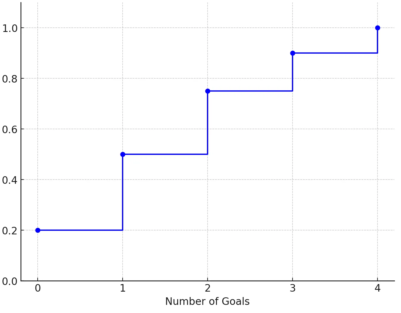
2.2. Cumulative Distribution Function (CDF)

The Cumulative Distribution Function (CDF) is a fundamental concept in probability theory and statistics that describes the probability that a random variable takes on a value less than or equal to a specific value. It provides a complete description of the distribution of a random variable.

For a given random variable \(X\), the Cumulative Distribution Function \(F_X(x)\) is defined as:

\[ F_X(x) = P(X \leq x) \]

This means that \(F_X(x)\) gives the probability that the random variable \(X\) will take a value less than or equal to \(x\).

– The CDF is a non-decreasing function. This means that as \(x\) increases, \(F_X(x)\) either stays the same or increases.

– The CDF ranges between 0 and 1.

– The CDF is always right-continuous, meaning that there are no sudden jumps when you approach a point from the right.

– If \(X\) is a continuous random variable, the derivative of the CDF with respect to \(x\) gives the Probability Density Function (PDF)

\[ f_X(x) = \frac{d}{dx} F_X(x) \]

Let’s see a basic example. Imagine you’re analyzing the number of goals a football team scores in a match. Over the course of a season, you’ve observed the following distribution of goals scored per match:

• 0 goals: 20% of matches => P(X = 0) = 0.2
• 1 goal: 30% of matches => P(X = 1) = 0.3
• 2 goals: 25% of matches => P(X = 2) = 0.25
• 3 goals: 15% of matches => P(X = 3) = 0.15
• 4 goals: 10% of matches => P(X = 4) = 0.1

The CDF gives us the probability that the number of goals scored is less than or equal to a certain number

• F(0) = P(X <= 0) = 0.2 => There is a 20% chance that the team will score 0 goals or less (which in this case means exactly 0 goals).
• F(1) = P(X <= 1) = P(X = 0) + P(X = 1) = 0.2 + 0.3 = 0.5 => There is a 50% chance that the team will score 1 goal or less.
• F(2) = P(X <= 2) = P(X <= 1) + P(X = 2) = 0.5 + 0.25 = 0.75 => There is a 75% chance that the team will score 2 goals or less.
• F(3) = P(X <= 3) = P(X <= 2) + P(X = 3) = 0.75 + 0.15 = 0.9 => There is a 90% chance that the team will score 3 goals or less.
• F(4) = P(X <= 4) = P(X <= 3) + P(X = 4) = 0.9 + 0.1 = 1 => There is a 100% chance that the team will score 4 goals or less.