Kien Duong

December 6, 2024

Recurrent Neural Network (RNN)

Recurrent Neural Network (RNN) is a type of artificial neural network designed for processing sequential data. The main differences between a RNN and a traditional feedforward neural network revolve around how they process data, especially with respect to sequential and temporal data.

1. Forward Pass

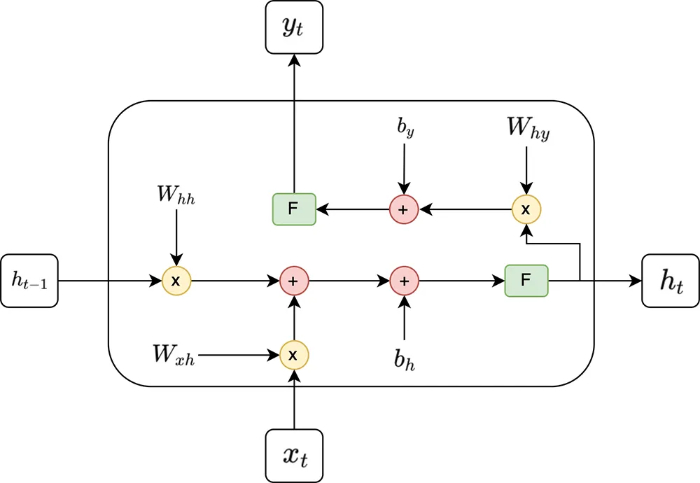
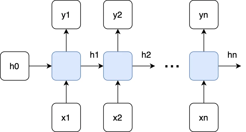
At each time step $t$, the RNN takes an input $x_t$ and updates its hidden state $h_t$ using the previous hidden state $h_{t-1}$. The hidden state is then used to generate an output $y_t$.

1.1. Hidden state

\[ h_t = \sigma(W_{xh}x_t + W_{hh}h_{t-1} + b_h) \]

$$h_t$$ : The hidden state at time $t$
$W_{xh}$: The weight matrix for the input
$W_{hh}$: The weight matrix for the previous hidden state
: The bias term
$\sigma$ : Activation function (often a non-linear function like tanh or ReLU)
$x_t$ : The input at time step $t$
: The hidden state at the previous time step

1.2. Output

\[ y_t = \phi(W_{hy}h_t + b_y) \]

$$y_t$$ : The output at time $t$
: The weight matrix from the hidden state to the output
$b_y$ : The bias term for the output
$\phi$ : Activation function (such as softmax for classification problems)

1. A time step

2. Many time steps

2. Total Loss

\[ \mathcal{L} = \sum_{t=1}^{T} \text{Loss}_t \]

$Loss_t$ is the difference between the predicted output $y_t$ and the actual target $\hat{y}_t$ for that time step. The formula for $Loss_t$ depends on the specific task and loss function being used.

3. Backpropagation Through Time (BPTT)

In RNN, the hidden state at each time step depends on the hidden states from previous time steps. It means that the error at a particular time step might influence errors at previous time steps. So the gradients must be propagated backward through these time steps.

During backpropagation, the goal is to compute the gradients of the loss with respect to the parameters $W_{xh}$

3.1. Input to Hidden

\[ \frac{\partial \mathcal{L}}{\partial W_{xh}} = \sum_{t=1}^{T} \frac{\partial \mathcal{L}_t}{\partial h_t} \cdot \frac{\partial h_t}{\partial W_{xh}} \]

3.2. Hidden to Hidden

\[ \frac{\partial \mathcal{L}}{\partial W_{hh}} = \sum_{t=1}^{T} \sum_{k=1}^{t} \frac{\partial \mathcal{L}_t}{\partial h_t} \cdot \frac{\partial h_t}{\partial h_k} \cdot \frac{\partial h_k}{\partial W_{hh}} \]

The inner sum $\sum_{k=1}^{t}$ accumulates the contribution of all previous hidden states $h_k$ (from $k = 1$ to $k = t$) that influenced the current hidden state $h_t$. This is necessary because each hidden state in the RNN influences all subsequent hidden states.
The outer sum $\sum_{t=1}^{T}$ goes over all time steps in the sequence from $t = 1$ to $T$, which is the length of the input sequence. For each time step $t$, we compute how the loss $\mathcal{L}_t$ at that time depends on the hidden-to-hidden weights.

3.3. Hidden to Output

\[ \frac{\partial \mathcal{L}}{\partial W_{hy}} = \sum_{t=1}^{T} \frac{\partial \mathcal{L}_t}{\partial y_t} \cdot \frac{\partial y_t}{\partial W_{hy}} \]

3.4. Hidden State Bias

\[ \frac{\partial \mathcal{L}}{\partial b_h} = \sum_{t=1}^{T} \frac{\partial \mathcal{L}_t}{\partial h_t} \cdot \frac{\partial h_t}{\partial b_h} \]

3.5. Output Bias

\[ \frac{\partial \mathcal{L}}{\partial b_y} = \sum_{t=1}^{T} \frac{\partial \mathcal{L}_t}{\partial y_t} \cdot \frac{\partial y_t}{\partial b_y} \]

3.6. Update the weights

The parameters (weights and biases) are updated using an optimization algorithm like Stochastic Gradient Descent (SGD)

\[ W_{xh} = W_{xh} – \eta \cdot \frac{\partial \mathcal{L}}{\partial W_{xh}} \]

\[ W_{hh} = W_{hh} – \eta \cdot \frac{\partial \mathcal{L}}{\partial W_{hh}} \]

\[ W_{hy} = W_{hy} – \eta \cdot \frac{\partial \mathcal{L}}{\partial W_{hy}} \]

\[ b_h = b_h – \eta \cdot \frac{\partial \mathcal{L}}{\partial b_h} \]

\[ b_y = b_y – \eta \cdot \frac{\partial \mathcal{L}}{\partial b_y} \]

$\eta$ is the learning rate

4. Basic example

Predicting the outcome: Goal, Save, Miss based on a sequence of actions: Pass, Dribble, Shot.

4.1. RNN architecture

The actions: [Pass, Dribble, Shot, Goal, Save, Miss]

Pass: [1,0,0,0,0,0]
Dribble: [0,1,0,0,0,0]
Shot: [0,0,1,0,0,0]
Goal: [0,0,0,1,0,0]
Save: [0,0,0,0,1,0]
Miss: [0,0,0,0,0,1]

Hidden states size: 3

Input size: 6 (possible actions)

Output size: 3 (Goal, Save, Miss)

4.2. Weights & Bias

Assume the following parameters:

$W_{xh}$

\[ W_{xh} = \begin{bmatrix} 0.1 & 0.2 & 0.3 \\ 0.4 & 0.5 & 0.6 \\ 0.7 & 0.8 & 0.9 \\ 0.2 & 0.3 & 0.4 \\ 0.1 & 0.1 & 0.1 \\ 0.3 & 0.2 & 0.1 \end{bmatrix} \]

$W_{hh}$

\[ W_{hh} = \begin{bmatrix} 0.1 & 0.2 & 0.3 \\ 0.4 & 0.5 & 0.6 \\ 0.7 & 0.8 & 0.9 \end{bmatrix} \]

$ b_h $

\[ b_h = \begin{bmatrix} 0.1 \\ 0.1 \\ 0.1 \end{bmatrix} \]

$ W_{hy} $

\[ W_{hy} = \begin{bmatrix} 0.2 & 0.1 & 0.3 \\ 0.3 & 0.4 & 0.5 \\ 0.6 & 0.7 & 0.8 \end{bmatrix} \]

$b_y$

\[ b_y = \begin{bmatrix} 0.1 \\ 0.1 \\ 0.1 \end{bmatrix} \]

4.3. Hidden states

For each time step $t$, compute the hidden state $h_t$ using:

\[ h_t = \tanh(W_{xh} x_t + W_{hh} h_{t-1} + b_h) \]

4.4. Output

At the final step, compute the output $y_t$ using:

\[ y_t = \text{softmax}(W_{hy} h_t + b_y) \]

4.5. Calculation

For example, we have the sequence: Pass -> Dribble -> Shot

At time step 1: Pass

\[ h_1 = \tanh\left(\begin{bmatrix} 0.1 & 0.2 & 0.3 \\ 0.4 & 0.5 & 0.6 \\ 0.7 & 0.8 & 0.9 \\ 0.2 & 0.3 & 0.4 \\ 0.1 & 0.1 & 0.1 \\ 0.3 & 0.2 & 0.1 \end{bmatrix}
\begin{bmatrix} 1 \\ 0 \\ 0 \\ 0 \\ 0 \\ 0 \end{bmatrix} +
\begin{bmatrix} 0.1 & 0.2 & 0.3 \\ 0.4 & 0.5 & 0.6 \\ 0.7 & 0.8 & 0.9 \end{bmatrix}
\begin{bmatrix} 0 \\ 0 \\ 0 \end{bmatrix} +
\begin{bmatrix} 0.1 \\ 0.1 \\ 0.1 \end{bmatrix}\right) \]

\[ \Rightarrow h_1 = \begin{bmatrix} 0.197 \\ 0.462 \\ 0.664 \end{bmatrix} \]

\[ \Rightarrow y_1 = \text{softmax}\left(\begin{bmatrix} 0.2 & 0.1 & 0.3 \\ 0.3 & 0.4 & 0.5 \\ 0.6 & 0.7 & 0.8 \end{bmatrix}
\begin{bmatrix} 0.197 \\ 0.462 \\ 0.664 \end{bmatrix} + \begin{bmatrix} 0.1 \\ 0.1 \\ 0.1 \end{bmatrix}\right) \]

\[ \Rightarrow y_1 = \begin{bmatrix} 0.231 \\ 0.309 \\ 0.460 \end{bmatrix} \]

23.1% chance of Goal.

30.9% chance of Save.

46.0% chance of Miss.

At time step 2: Dribble

\[ h_2 = \tanh\left(\begin{bmatrix} 0.1 & 0.2 & 0.3 \\ 0.4 & 0.5 & 0.6 \\ 0.7 & 0.8 & 0.9 \\ 0.2 & 0.3 & 0.4 \\ 0.1 & 0.1 & 0.1 \\ 0.3 & 0.2 & 0.1 \end{bmatrix}
\begin{bmatrix} 0 \\ 1 \\ 0 \\ 0 \\ 0 \\ 0 \end{bmatrix} +
\begin{bmatrix} 0.1 & 0.2 & 0.3 \\ 0.4 & 0.5 & 0.6 \\ 0.7 & 0.8 & 0.9 \end{bmatrix}
\begin{bmatrix} 0.197 \\ 0.462 \\ 0.664 \end{bmatrix} +
\begin{bmatrix} 0.1 \\ 0.1 \\ 0.1 \end{bmatrix}\right) \]

\[ \Rightarrow h_2 = \begin{bmatrix} 0.547 \\ 0.869 \\ 0.967 \end{bmatrix} \]

\[ \Rightarrow y_2 = \text{softmax}\left(\begin{bmatrix} 0.2 & 0.1 & 0.3 \\ 0.3 & 0.4 & 0.5 \\ 0.6 & 0.7 & 0.8 \end{bmatrix}
\begin{bmatrix} 0.547 \\ 0.869 \\ 0.967 \end{bmatrix} + \begin{bmatrix} 0.1 \\ 0.1 \\ 0.1 \end{bmatrix}\right) \]
\[ \Rightarrow y_2 = \begin{bmatrix} 0.165 \\ 0.274 \\ 0.561 \end{bmatrix} \]

16.5% chance of Goal.

27.4% chance of Save.

56.1% chance of Miss.

At time step 3: Shot

\[ h_3 = \tanh\left(\begin{bmatrix} 0.1 & 0.2 & 0.3 \\ 0.4 & 0.5 & 0.6 \\ 0.7 & 0.8 & 0.9 \\ 0.2 & 0.3 & 0.4 \\ 0.1 & 0.1 & 0.1 \\ 0.3 & 0.2 & 0.1 \end{bmatrix}
\begin{bmatrix} 0 \\ 0 \\ 1 \\ 0 \\ 0 \\ 0 \end{bmatrix} +
\begin{bmatrix} 0.1 & 0.2 & 0.3 \\ 0.4 & 0.5 & 0.6 \\ 0.7 & 0.8 & 0.9 \end{bmatrix}
\begin{bmatrix} 0.547 \\ 0.869 \\ 0.967 \end{bmatrix} +
\begin{bmatrix} 0.1 \\ 0.1 \\ 0.1 \end{bmatrix}\right) \]

\[ \Rightarrow h_3 = \begin{bmatrix} 0.784 \\ 0.975 \\ 0.997 \end{bmatrix} \]

\[ \Rightarrow y_3 = \text{softmax}\left(\begin{bmatrix} 0.2 & 0.1 & 0.3 \\ 0.3 & 0.4 & 0.5 \\ 0.6 & 0.7 & 0.8 \end{bmatrix}
\begin{bmatrix} 0.784 \\ 0.975 \\ 0.997 \end{bmatrix} +
\begin{bmatrix} 0.1 \\ 0.1 \\ 0.1 \end{bmatrix}\right) \]

\[ \Rightarrow y_3 = \begin{bmatrix} 0.147 \\ 0.260 \\ 0.593 \end{bmatrix} \]

14.7% chance of Goal.

26.0% chance of Save.

59.3% chance of Miss.

4.6. Pytorch code

    import torch

# Define the params
W_xh = torch.tensor([[0.1, 0.2, 0.3], [0.4, 0.5, 0.6], [0.7, 0.8, 0.9],
                     [0.2, 0.3, 0.4], [0.1, 0.1, 0.1], [0.3, 0.2, 0.1]], dtype=torch.float32)

W_hh = torch.tensor([[0.1, 0.2, 0.3],
                     [0.4, 0.5, 0.6],
                     [0.7, 0.8, 0.9]], dtype=torch.float32)

W_hy = torch.tensor([[0.2, 0.1, 0.3],
                     [0.3, 0.4, 0.5],
                     [0.6, 0.7, 0.8]], dtype=torch.float32)

b_h = torch.tensor([0.1, 0.1, 0.1], dtype=torch.float32)
b_y = torch.tensor([0.1, 0.1, 0.1], dtype=torch.float32)

# Input sequence: "Pass", "Dribble", "Shot"
x_seq = [
    torch.tensor([1, 0, 0, 0, 0, 0], dtype=torch.float32),
    torch.tensor([0, 1, 0, 0, 0, 0], dtype=torch.float32),
    torch.tensor([0, 0, 1, 0, 0, 0], dtype=torch.float32)
]

h_0 = torch.tensor([0.0, 0.0, 0.0], dtype=torch.float32)

# Calculate hidden state
def calculate_hidden_state(W_xh, W_hh, x_t, h_prev, b_h):
    return torch.tanh(torch.matmul(W_xh.T, x_t) + torch.matmul(W_hh, h_prev) + b_h)

# Calculate output
def calculate_output(W_hy, h_t, b_y):
    z_t = torch.matmul(W_hy, h_t) + b_y
    y_t = torch.softmax(z_t, dim=0)
    return y_t

h_t = h_0
hidden_states = []
outputs = []

for x_t in x_seq:
    h_t = calculate_hidden_state(W_xh, W_hh, x_t, h_t, b_h)
    hidden_states.append(h_t.clone())
    y_t = calculate_output(W_hy, h_t, b_y)
    outputs.append(y_t)

for i, (h_t, y_t) in enumerate(zip(hidden_states, outputs), 1):
    print(f"Time step {i}:")
    print(f"h_{i}: {h_t}")
    print(f"y_{i}: {y_t}")
    print()

The result is:

    Time step 1:
h_1: tensor([0.1974, 0.2913, 0.3799])
y_1: tensor([0.2660, 0.3195, 0.4146])

Time step 2:
h_2: tensor([0.5993, 0.7828, 0.8882])
y_2: tensor([0.1732, 0.2778, 0.5490])

Time step 3:
h_3: tensor([0.8573, 0.9683, 0.9933])
y_3: tensor([0.1446, 0.2569, 0.5985])

5. RNN with Pytorch

5.1. Dataset

Input Sequence	Target Outcome
[“Pass”, “Dribble”, “Shot”]	“Goal”
[“Dribble”, “Shot”, “Save”]	“Save”
[“Pass”, “Pass”, “Miss”]	“Miss”
[“Dribble”, “Shot”, “Goal”]	“Goal”
[“Pass”, “Dribble”, “Save”]	“Save”

5.2. Pytorch code

    import torch
import torch.nn as nn
import torch.optim as optim

# Define the dataset
action_to_index = {"Pass": 0, "Dribble": 1, "Shot": 2, "Goal": 3, "Save": 4, "Miss": 5}
index_to_action = {v: k for k, v in action_to_index.items()}

# Training sequences and targets
sequences = [
    ["Pass", "Dribble", "Shot"],
    ["Dribble", "Shot", "Save"],
    ["Pass", "Pass", "Miss"],
    ["Dribble", "Shot", "Goal"],
    ["Pass", "Dribble", "Save"]
]

targets = ["Goal", "Save", "Miss", "Goal", "Save"]

def encode_sequence(sequence, action_to_index):
    one_hot = torch.zeros(len(sequence), len(action_to_index))
    for i, action in enumerate(sequence):
        one_hot[i][action_to_index[action]] = 1.0
    return one_hot

def encode_target(target, action_to_index):
    return torch.tensor(action_to_index[target])

encoded_sequences = [encode_sequence(seq, action_to_index) for seq in sequences]
encoded_targets = [encode_target(t, action_to_index) for t in targets]

# Define the RNN model
class RNN(nn.Module):
    def __init__(self, input_size, hidden_size, output_size):
        super(RNN, self).__init__()
        self.hidden_size = hidden_size
        self.rnn = nn.RNN(input_size, hidden_size, batch_first=True)
        self.fc = nn.Linear(hidden_size, output_size)

    def forward(self, x, h):
        out, h = self.rnn(x, h)
        out = self.fc(out[:, -1, :])  # Only take the last output
        return out, h

input_size = len(action_to_index)
hidden_size = 8
output_size = len(action_to_index)
learning_rate = 0.01
num_epochs = 100

# Initialize the model, loss, and optimizer
model = RNN(input_size, hidden_size, output_size)
criterion = nn.CrossEntropyLoss()
optimizer = optim.Adam(model.parameters(), lr=learning_rate)

# Training loop
for epoch in range(num_epochs):
    total_loss = 0
    for seq, target in zip(encoded_sequences, encoded_targets):
        seq = seq.unsqueeze(0)  # Add batch dimension
        target = target.unsqueeze(0)

        # Initialize hidden state
        h = torch.zeros(1, 1, hidden_size)

        # Forward pass
        output, h = model(seq, h)
        loss = criterion(output, target)

        # Backward pass and optimization
        optimizer.zero_grad()
        loss.backward()
        optimizer.step()

        total_loss += loss.item()

    if (epoch + 1) % 10 == 0:
        print(f"Epoch [{epoch + 1}/{num_epochs}], Loss: {total_loss:.4f}")

# Evaluate the model
def predict(sequence):
    with torch.no_grad():
        seq = encode_sequence(sequence, action_to_index).unsqueeze(0)
        h = torch.zeros(1, 1, hidden_size)
        output, h = model(seq, h)
        prediction = torch.argmax(output, dim=1).item()
        return index_to_action[prediction]

# Test the model
test_sequence = ["Pass", "Dribble", "Shot"]
prediction = predict(test_sequence)
print(f"Input: {test_sequence}, Predicted Outcome: {prediction}")

The result is:

    Epoch [10/100], Loss: 3.5789
Epoch [20/100], Loss: 0.9481
Epoch [30/100], Loss: 0.3500
Epoch [40/100], Loss: 0.1914
Epoch [50/100], Loss: 0.1247
Epoch [60/100], Loss: 0.0894
Epoch [70/100], Loss: 0.0680
Epoch [80/100], Loss: 0.0538
Epoch [90/100], Loss: 0.0439
Epoch [100/100], Loss: 0.0367
Input: ['Pass', 'Dribble', 'Shot'], Predicted Outcome: Goal