Singular Value Decomposition (SVD)

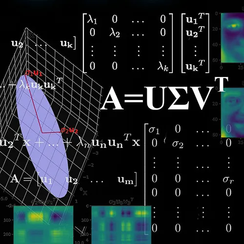
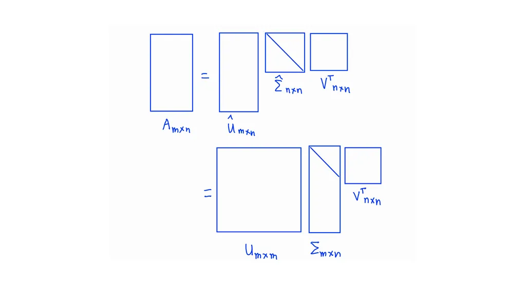
1. What is SVD?

The SVD of a matrix A is the factorization of A into the product of three matrices.

$$
\mathbf{A}_{m \times n} = \mathbf{U}_{m \times m} \mathbf{\Sigma}_{m \times n} (\mathbf{V}_{n \times n})^T
$$

\(\mathbf{U}, \mathbf{V}\) are orthogonal matrices. \(\mathbf{\Sigma}\) is diagonal matrix.

Let’s see a simple example

$$
\mathbf{x} =
\begin{bmatrix}
1 \\
3
\end{bmatrix}
~~~
\mathbf{A} =
\begin{bmatrix}
2 & 1 \\
-1 & 1
\end{bmatrix}
$$

$$
\Rightarrow
\mathbf{y} = \mathbf{A} \mathbf{x} =
\begin{bmatrix}
2 & 1 \\
-1 & 1
\end{bmatrix}
\begin{bmatrix}
1 \\
3
\end{bmatrix} =
\begin{bmatrix}
5 \\
2
\end{bmatrix}
$$

Based on the graph, we can see the transformation from vector \(\mathbf{x}\) to vector \(\mathbf{y}\) includes two actions: “rotating” & “stretching”.

For the next step, we have an orthogonal matrix \(\mathbf{V}_{2 \times 2}\) and a matrix \(\mathbf{A}_{m \times n}\). The transformation should be:

\(\mathbf{u}_{1}\), \(\mathbf{u}_{2}\) are unit orthonormal vectors. \(\mathbf{\sigma}_{1}\), \(\mathbf{\sigma}_{2}\) are “stretching”. So now, we have \(\mathbf{A} \mathbf{v}_{1} = \mathbf{\sigma}_{1}\mathbf{u}_{1}\). When \(\mathbf{v} \in \mathbb{R}^{n \times n} \), the formula should be:

$$
\mathbf{A} \mathbf{v}_{j} = \mathbf{\sigma}_{j} \mathbf{u}_{j} ~~~~~ j = 1,2,3,…,n
$$

$$
\begin{align}
A
\begin{bmatrix}
\mathbf{v_1} & \mathbf{v_2} & \dots & \mathbf{v_n}
\end{bmatrix}
&=
\begin{bmatrix}
\mathbf{u_1} & \mathbf{u_2} & \dots & \mathbf{u_n}
\end{bmatrix}
\begin{bmatrix}
\sigma_{1} & 0 & \dots & 0 \\
0 & \sigma_{2} &\dots & 0 \\
\vdots & \vdots & \ddots & \vdots \\
0 & 0 & \dots & \sigma_{n} \\
\end{bmatrix} \\
AV &= U\Sigma
\end{align}
$$

Because \(\mathbf{V}\) is an orthogonal matrix so \(\mathbf{V}^{-1} = \mathbf{V}^{T}\). Therefore the formular is:

$$
\begin{align}
AV &= U\Sigma \\
\Rightarrow AVV^{-1} &= U{\Sigma}V^{-1} \\
\Rightarrow AI &= U{\Sigma}V^{T} \\
\Rightarrow A &= U{\Sigma}V^{T} \\
\end{align}
$$

Theorem: Every matrix \(\mathbf{A} \in \mathbb{R}^{m \times n} \) has a Singular Value Decomposition (SVD)

Reference: https://www.cs.princeton.edu/courses/archive/spring12/cos598C/svdchapter.pdf

2. Eigen Decomposition

Given a matrix \(\mathbf{A}\), if we can find \(\lambda\) and \(\mathbf{v}\) satisfying the below equation so \(\mathbf{v}\) is eigenvector & \(\lambda\) is eigenvalue of \(\mathbf{A}\)

$$
\begin{align}
\mathbf{A} \mathbf{v} &= \lambda \mathbf{v} \\
\Rightarrow (\mathbf{A} – \lambda\mathbf{I})\mathbf{v} &= 0
\end{align}
$$

Back to SVD, we have

$$
\begin{align}
AA^T &= U{\Sigma}V^{T} (U{\Sigma}V^{T})^{T} \\
&= U{\Sigma}V^T V{\Sigma}^TU^T \\
&= U{\Sigma}{\Sigma}^TU^T \\
\Rightarrow AA^TU &= U{\Sigma}{\Sigma}^TU^TU \\
&= U{\Sigma}{\Sigma}^T ~~~~~~~~ (2.1)
\end{align}
$$

$$
\begin{align}
A^TA &= (U{\Sigma}V^{T})^{T}U{\Sigma}V^{T} \\
&= V{\Sigma}^TU^TU{\Sigma}V^T \\
&= V{\Sigma}^T{\Sigma}V^T \\
\Rightarrow A^TAV &= V{\Sigma}^T{\Sigma}V^TV \\
&= V{\Sigma}^T{\Sigma} ~~~~~~~~ (2.2)
\end{align}
$$

From (2.1) we have \(U\) is eigenvector and \({\Sigma}{\Sigma}^T\) is eigenvalue of \(AA^T\). We can see that \({\Sigma}{\Sigma}^T\) is a diagonal matrix that has main diagonal elements are \(\sigma_1^2, \sigma_2^2,…\).

Similarly, from (2.2) we have \(V\) is eigenvector and \({\Sigma}^T{\Sigma}\) is eigenvalue of \(A^TA\).

3. Find SVD manually

3.1. Find left singular vector U

$$
\begin{align}
A &=
\begin{bmatrix}
3 & 2 & 2 \\
2 & 3 & -2
\end{bmatrix} \\
\Rightarrow AA^T &=
\begin{bmatrix}
3 & 2 & 2 \\
2 & 3 & -2
\end{bmatrix}
\begin{bmatrix}
3 & 2 \\
2 & 3 \\
2 & -2
\end{bmatrix} \\
&=
\begin{bmatrix}
17 & 8 \\
8 & 17
\end{bmatrix} \\
\Rightarrow AA^T – \lambda I &=
\begin{bmatrix}
17 & 8 \\
8 & 17
\end{bmatrix} –
\begin{bmatrix}
\lambda & 0 \\
0 & \lambda
\end{bmatrix} \\
&=
\begin{bmatrix}
17 – \lambda & 8 \\
8 & 17 – \lambda
\end{bmatrix} \\
\Rightarrow det(AA^T – \lambda I) &=
(17 – \lambda)^2 – 64 \\
&= \lambda^2 – 34 \lambda + 225 \\
&= (\lambda – 25)(\lambda – 9) ~~~~~~~~~~~~ (3.1)
\end{align}
$$

The equation (3.1) has 2 solutions \(\lambda = 25\) and \(\lambda = 9\)

3.1.1 \(\lambda = 25\)

$$
\begin{align}
AA^T – \lambda I &=
\begin{bmatrix}
17 – \lambda & 8 \\
8 & 17 – \lambda
\end{bmatrix} \\
&=
\begin{bmatrix}
-8 & 8 \\
8 & -8
\end{bmatrix}
\end{align}
$$

Using the elimination method to row reduce that matrix

$$
\begin{align}
\begin{bmatrix}
-8 & 8 \\
8 & -8
\end{bmatrix}
\Rightarrow
\begin{bmatrix}
1 & -1 \\
1 & -1
\end{bmatrix}
\Rightarrow
\begin{bmatrix}
1 & -1 \\
0 & 0
\end{bmatrix}
\Rightarrow
x – y = 0
\Rightarrow
x = y
\end{align}
$$

The next step, we will find the unit vector. Unit vector is a vector that has magnitude is exactly 1 unit.

$$
\begin{align}
\sqrt{x^2 + y^2} = 1
\Rightarrow
x^2 + y^2 = 1
\Rightarrow
2x^2 = 1
\Rightarrow
x = y = \frac{1}{\sqrt{2}}
\end{align}
$$

So the first vector of \(U\) should be

$$
u_1 =
\begin{bmatrix}
\frac{1}{\sqrt{2}} \\
\frac{1}{\sqrt{2}}
\end{bmatrix}
$$

3.1.2 \(\lambda = 9\)

Similar to the above we can calculate the second vector of \(U\) should be

$$
u_2 =
\begin{bmatrix}
\frac{1}{\sqrt{2}} \\
-\frac{1}{\sqrt{2}}
\end{bmatrix}
$$

So

$$
U =
\begin{bmatrix}
\frac{1}{\sqrt{2}} && \frac{1}{\sqrt{2}} \\
\frac{1}{\sqrt{2}} && -\frac{1}{\sqrt{2}}
\end{bmatrix}
$$

3.2. Find right singular vector V

$$
\begin{align}
A &=
\begin{bmatrix}
3 & 2 & 2 \\
2 & 3 & -2
\end{bmatrix} \\
\Rightarrow A^TA &=
\begin{bmatrix}
3 & 2 \\
2 & 3 \\
2 & -2
\end{bmatrix}
\begin{bmatrix}
3 & 2 & 2 \\
2 & 3 & -2
\end{bmatrix} \\
&=
\begin{bmatrix}
13 & 12 & 2 \\
12 & 13 & -2 \\
2 & -2 & 8
\end{bmatrix}
\end{align}
$$

3.2.1. \(\lambda = 25\)

$$
\begin{align}
A^TA – \lambda I &=
\begin{bmatrix}
13 – \lambda & 12 & 2 \\
12 & 13 – \lambda & -2 \\
2 & -2 & 8 – \lambda
\end{bmatrix} \\
&=
\begin{bmatrix}
-12 & 12 & 2 \\
12 & -12 & -2 \\
2 & -2 & -17
\end{bmatrix}
\end{align}
$$

That vector row reduces to

$$
\begin{bmatrix}
1 & -1 & 0 \\
0 & 0 & 1 \\
0 & 0 & 0
\end{bmatrix}
$$

So the first vector of \(V\) should be

$$
v_1 =
\begin{bmatrix}
\frac{1}{\sqrt{2}} \\
\frac{1}{\sqrt{2}} \\
0
\end{bmatrix}
$$

3.2.2. \(\lambda = 9\)

So the second vector of \(V\) should be

$$
v_2 =
\begin{bmatrix}
\frac{1}{\sqrt{18}} \\
-\frac{1}{\sqrt{18}} \\
\frac{4}{\sqrt{18}}
\end{bmatrix}
$$

3.2.3. Find last eigenvector

As above, we already find the eigenvectors \(v_1\) & \(v_2\) of orthogonal matrix \(V\). So now, we need to find the eigenvector \(v_3\). Based on the properties of orthonormal vectors. We have:

$$
v_3 =
\begin{bmatrix}
a \\
b \\
c
\end{bmatrix}
$$

$$
\begin{align}
\frac{a}{\sqrt{2}} + \frac{b}{\sqrt{2}} + 0 c &= 0 \\
\Rightarrow b &= -a
\end{align}
$$

$$
\begin{align}
\frac{a}{\sqrt{18}} – \frac{b}{\sqrt{18}} + \frac{4c}{\sqrt{18}} &= 0 \\
\Rightarrow c &= -\frac{a}{2}
\end{align}
$$

The next step, we find the unit vector

$$
\begin{align}
a^2 + b^2 + c^2 &= 1 \\
\Rightarrow
a^2 + (-a)^2 + (-\frac{a}{2})^2 &= 1 \\
\Rightarrow
a &= \frac{2}{3} \\
\Rightarrow
v_3 &=
\begin{bmatrix}
\frac{2}{3} \\
\frac{-2}{3} \\
\frac{-1}{3}
\end{bmatrix}
\end{align}
$$

So

$$
V =
\begin{bmatrix}
\frac{1}{\sqrt{2}} & \frac{1}{\sqrt{18}} & \frac{2}{3} \\
\frac{1}{\sqrt{2}} & \frac{-1}{\sqrt{18}} & \frac{-2}{3} \\
0 & \frac{4}{\sqrt{18}} & \frac{-1}{3}
\end{bmatrix} \\
$$

$$
\Rightarrow
A = U \Sigma V^T =
\begin{bmatrix}
\frac{1}{\sqrt{2}} & \frac{1}{\sqrt{2}} \\
\frac{1}{\sqrt{2}} & -\frac{1}{\sqrt{2}}
\end{bmatrix}
\begin{bmatrix}
5 & 0 & 0 \\
0 & 3 & 0
\end{bmatrix}
\begin{bmatrix}
\frac{1}{\sqrt{2}} & \frac{1}{\sqrt{2}} & 0 \\
\frac{1}{\sqrt{18}} & \frac{-1}{\sqrt{18}} & \frac{4}{\sqrt{18}} \\
\frac{2}{3} & \frac{-2}{3} & \frac{-1}{3}
\end{bmatrix}
$$

4. Compute SVD by using Pytorch

PyTorch is a machine learning framework based on the Torch library, used for applications such as computer vision and natural language processing, originally developed by Meta AI.

Here is the Pytorch method to compute SVD: https://pytorch.org/docs/stable/generated/torch.svd.html Let’s write some basic code to compute SVD by a given matrix that based on above example:

The result: