Vanishing Gradient

The vanishing gradient problem in Recurrent Neural Network is a common issue that arises when training RNN using gradient optimization techniques. It occurs when the gradients of the loss function become too small to effectively update the weights. This makes it difficult for the network to learn long-term dependencies.

1. The main reason

– Activation functions like sigmoid or tanh produce small derivatives (values near 0).

– When gradients are propagated backward through multiple layers, they are repeatedly multiplied by these small values, causing them to shrink exponentially.

– In deep networks, the chain rule of differentiation results in gradients being a product of many small derivatives. This exponential decay in gradient size leads to vanishing gradients.

2. Basic example

2.1. Network setup

A 2 layers neural network.

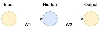
Sigmoid activation function.
\(x = 1\), \(W_1 = 0.5\), \(W_2 = 0.5\), \(y = 1\)

2.2. Forward Pass

2.2.1. First layer output

\[h = \sigma(W_1 \cdot x)\]

\[ \Rightarrow h = \sigma(0.5 \cdot 1) = \frac{1}{1 + e^{-0.5}} \approx 0.622 \]

2.2.2. Second layer output

\[ \hat{y} = \sigma(W_2 \cdot h) \]

\[ \Rightarrow \hat{y} = \sigma(0.5 \cdot 0.622) = \frac{1}{1 + e^{-0.311}} \approx 0.577 \]

2.2.3. Loss function

Use the Mean Squared Error (MSE):

\[ L = (\hat{y} – y)^2 \]

\[ \Rightarrow L = (0.577 – 1)^2 \approx 0.179 \]

2.3. Backward Pass

To update \(W_1\), we calculate the gradient by using the chain rule:

\[ \frac{\partial L}{\partial W_1} = \frac{\partial L}{\partial \hat{y}} \cdot \frac{\partial \hat{y}}{\partial h} \cdot \frac{\partial h}{\partial W_1} \]

2.3.1. Gradient of loss with respect to output

\[ \frac{\partial L}{\partial \hat{y}} = 2 (\hat{y} – y) \]

\[ \Rightarrow \frac{\partial L}{\partial \hat{y}} = 2 (0.577 – 1) = -0.846 \]

2.3.2. Gradient of \(\hat{y}\) with respect to \(h\)

\[ \frac{\partial \hat{y}}{\partial h} = \frac{\partial \hat{y}}{\partial z} \cdot \frac{\partial z}{\partial h} \]

Where \( z = W_2 \cdot h \)

\[ \Rightarrow \frac{\partial \hat{y}}{\partial h} = \sigma'(z) \cdot W_2 \]

See the derivative of sigmoid at here.

\[ \Rightarrow \sigma'(0.311) = 0.577 \cdot (1 – 0.577) \approx 0.244 \]

\[ \Rightarrow \frac{\partial \hat{y}}{\partial h} = 0.5 \cdot 0.244 = 0.122 \]

2.3.3. Gradient of \(h\) with respect to \(W_1\)

\[ \frac{\partial h}{\partial W_1} = \frac{\partial h}{\partial z} \cdot \frac{\partial z}{\partial W_1} \]

Where \( z = W_1 \cdot x \)

\[ \Rightarrow \frac{\partial h}{\partial W_1} = \sigma'(z) \cdot x \]

\[ \Rightarrow \sigma'(0.5) = 0.622 \cdot (1 – 0.622) \approx 0.235 \]

\[ \Rightarrow \frac{\partial h}{\partial W_1} = 0.235 \cdot 1 = 0.235 \]

2.3.4. Final gradient for \(W_1\)

2.4. Weight updates

In gradient-based optimization, the weights \(W_1\) are updated as:

\[ W_1 \leftarrow W_1 – \eta \cdot \frac{\partial L}{\partial W_1} \]

Where \(\eta\) is the learning rate.

\( \frac{\partial L}{\partial W_1} \approx -0.024 \) is very small, so the weight \(W_1\) barely changes. This means the earlier layers of the network learn very slowly or not at all. It is the reason for the vanishing gradient problem.